D2-Net Trained on MegaDepth Data

Find generic keypoints and their feature vectors in an image

Number of layers: 22 | Parameter count: 7,635,264 | Trained size: 31 MB |

Training Set Information

MegaDepth, consisting of 196 different locations reconstructed from COLMAP SfM/MVS with 130 thousand images. Of these 130 thousand photos, around one hundred thousand images are used for Euclidean depth data, and the remaining 30 thousand images are used to derive ordinal depth data.

Performance

This model achieves 74.2% accuracy for correctly localized queries with a distance threshold equal to one meter on the InLoc dataset.

Examples

Download Example Notebook

Open in Wolfram Cloud

Resource retrieval

Get the pre-trained net:

In[1]:=

Out[1]=

Evaluation function

Write an evaluation function to post-process the net output in order to obtain keypoint position, strength and features:

In[2]:=

$Options[netevaluate] = {MaxFeatures -> 50}; netevaluate[img_Image, opts : OptionsPattern[]] := Module[ {dims, featureMap, c, h, w, transposed, normalized, strengthArray, pos, scalex, scaley, keypointStr, keypointPos, keypointFeats}, dims = ImageDimensions[img]; featureMap = NetModel["D2-Net Trained on MegaDepth Data"][img]; {c, h, w} = Dimensions[featureMap]; transposed = Transpose[featureMap, {3, 1, 2}]; normalized = transposed/Map[Norm, transposed, {2}]; (* Matrix containing the strengths of each keypoint *) strengthArray = Map[Max, normalized, {2}]; (* Find positions of (up to) MaxFeatures strongest keypoints *) pos = Ordering[ Flatten@strengthArray, -Min[OptionValue[MaxFeatures], w*h]] - 1; pos = QuotientRemainder[#, w] + {1, 1} & /@ pos; (* matrix position *) (* From array positions to image keypoint positions *) {scalex, scaley} = N[dims/{w, h}]; keypointPos = {scalex*(#[[1]] - 0.5), scaley*(h - #[[2]] + 0.5)} & /@ Reverse /@ pos; (* Extract the features and strengths *) keypointFeats = Extract[normalized, pos]; keypointStr = Extract[strengthArray, pos]; {keypointPos, keypointStr, keypointFeats} ]$

Basic usage

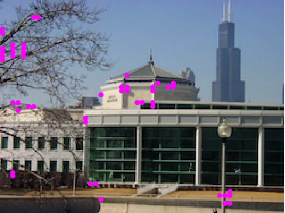
Obtain the keypoints of a given image:

In[3]:=

(* Evaluate this cell to get the example input *) CloudGet["https://www.wolframcloud.com/obj/ae785a2c-eb63-4af1-ad3c-70c6946b852b"]

In[4]:=

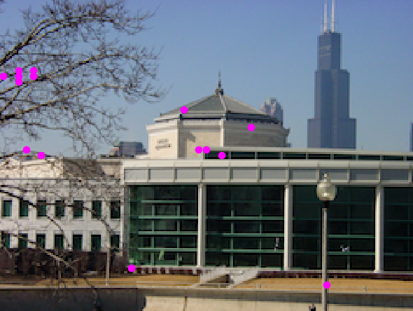
Visualize the keypoints:

In[5]:=

Out[5]=

Specify a maximum of 15 keypoints and visualize the new detection:

In[6]:=

In[7]:=

Out[7]=

Network result

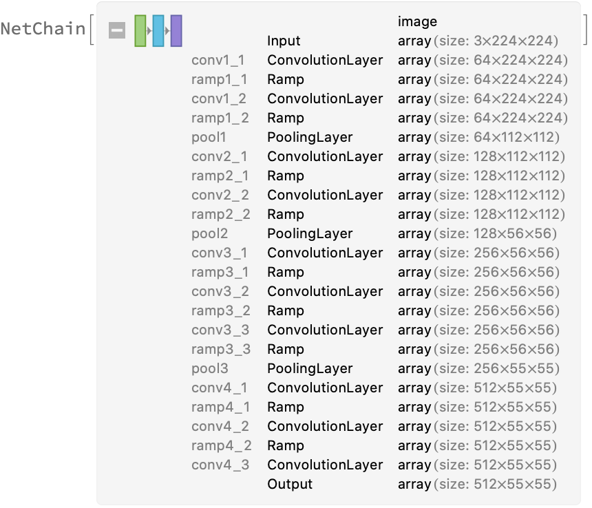
For the default input size of 224⨯224, the net divides the input image in 55⨯55 patches and computes a feature vector of size 512 for each patch:

In[8]:=

(* Evaluate this cell to get the example input *) CloudGet["https://www.wolframcloud.com/obj/085bf1db-e081-4a91-b16e-dc13c2f24cb7"]

In[9]:=

In[10]:=

Out[10]=

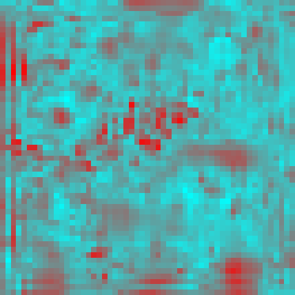
Every patch is associated to a scalar strength value indicating the likelihood that the patch contains a keypoint. The strength of each patch is the maximal element of its feature vector after an L2 normalization. Obtain the strength of each patch:

In[11]:=

strengthArray = With[{transposed = Transpose[netResult, {3, 1, 2}]},
Map[Max, transposed/Map[Norm, transposed, {2}], {2}]
];

Visualize the strength of each patch as a heat map:

In[12]:=

Out[12]=

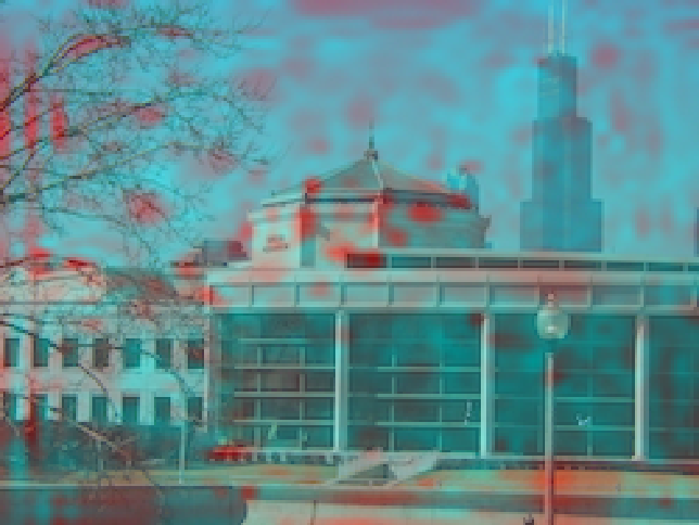
Overlay the heat map on the image:

In[13]:=

Out[13]=

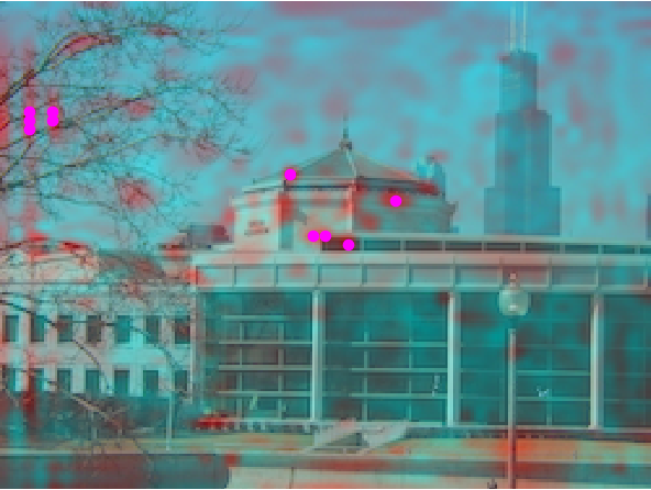
Keypoints are selected starting from the patch with highest strength, up to keypoints. Highlight the top 10 keypoints:

In[14]:=

In[15]:=

Out[15]=

Find correspondences between images

The main application of computing feature vectors for the image keypoints is to find correspondences in different images of the same scene. Get two hundred keypoint features from two images:

In[16]:=

(* Evaluate this cell to get the example input *) CloudGet["https://www.wolframcloud.com/obj/e0808678-8175-4e4d-89c9-6e3205aabbd9"]

In[17]:=

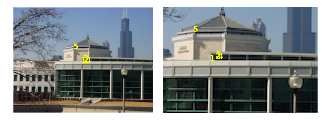
Define a function to find the n nearest pairs of keypoints (in feature space) and use it to find the five nearest pairs:

In[18]:=

$findKeypointPairs[feats1_, feats2_, n_] := Module[ {distances, nearestPairs, nearestDistances}, distances = DistanceMatrix[feats1, feats2]; nearestPairs = MapIndexed[Flatten@{#2, Ordering[#1, 1]} &, distances]; nearestDistances = Extract[distances, nearestPairs]; nearestPairs[[Ordering[nearestDistances, n]]] ];$

In[19]:=

Out[19]=

Get the keypoint positions associated with each pair and visualize them on the respective images:

In[20]:=

In[21]:=

GraphicsRow@MapThread[
Function[{img, keypoints},
Show[img, Graphics@
MapIndexed[Inset[Style[First@#2, 12, Yellow, Bold], #1] &, keypoints]]
],
{{img1, img2}, {pos1, pos2}}
]

Out[21]=

Net information

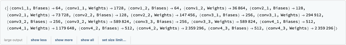
Inspect the number of parameters of all arrays in the net:

In[22]:=

Out[22]=

Obtain the total number of parameters:

In[23]:=

Out[23]=

Obtain the layer type counts:

In[24]:=

Out[24]=

Display the summary graphic:

In[25]:=

Out[25]=

Export to ONNX

Export the net to the ONNX format:

In[26]:=

Out[26]=

Get the size of the ONNX file:

In[27]:=

Out[27]=

The byte count of the resource object is similar to the ONNX file:

In[28]:=

Out[28]=

Check some metadata of the ONNX model:

In[29]:=

Out[29]=

Import the model back into the Wolfram Language. However, the NetEncoder and NetDecoder will be absent because they are not supported by ONNX:

In[30]:=

Out[30]=

Construction Notebook

Download Construction Notebook

Open in Wolfram Cloud

Resource History

Date Created: 22 September 2021

Reference

M. Dusmanu, I. Rocco, T. Pajdla, M. Pollefeys, J. Sivic, A. Torii, T. Sattler, "D2-Net: A Trainable CNN for Joint Detection and Description of Local Features," arXiv:1905.03561 (2019)
Available from: https://github.com/mihaidusmanu/d2-net
Rights: D2-net BSD license