CREPE Pitch Detection Net
Trained on
Monophonic Signal Data
Released in 2018, CREPE is a state-of-the-art system based on a deep convolutional neural network that operates directly on the time-domain waveform. The architecture is based on a chain of six convolution stacks, followed by a classifier. The net outputs a vector that represents the probability of the pitch being in one of 360 frequency classes nonlinearly spaced.
Number of layers: 41 |
Parameter count: 22,244,328 |
Trained size: 89 MB |
Examples
Resource retrieval
Get the pre-trained net:
Evaluation function
Define a Hidden Markov process that will be used for decoding the output of the net:
This net takes a monophonic audio signal and outputs an estimation of the pitch of the signal on a logarithmic pitch scale. Write an evaluation function to convert the result to a TimeSeries containing the predicted frequency in Hz and the confidence of the prediction:
Basic usage
Detect the pitch of a monophonic signal:
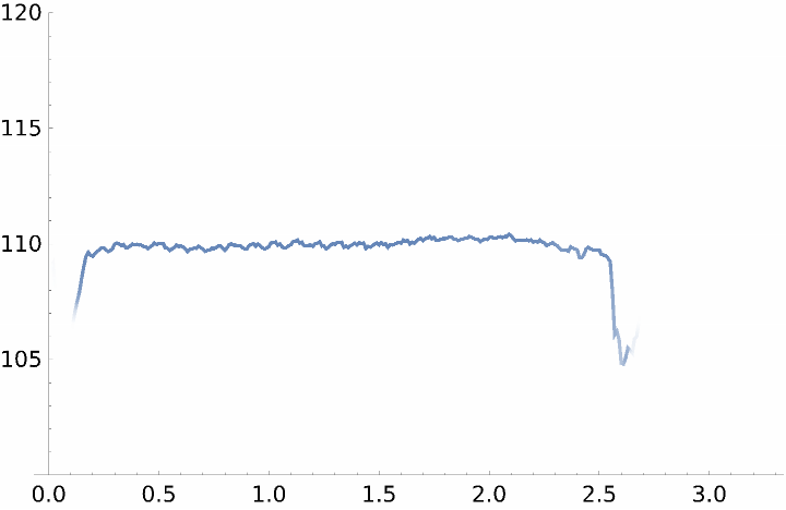
Plot the predicted frequency with the confidence mapped to the opacity:
Performance evaluation
Generate a signal using a sinusoidal oscillator:
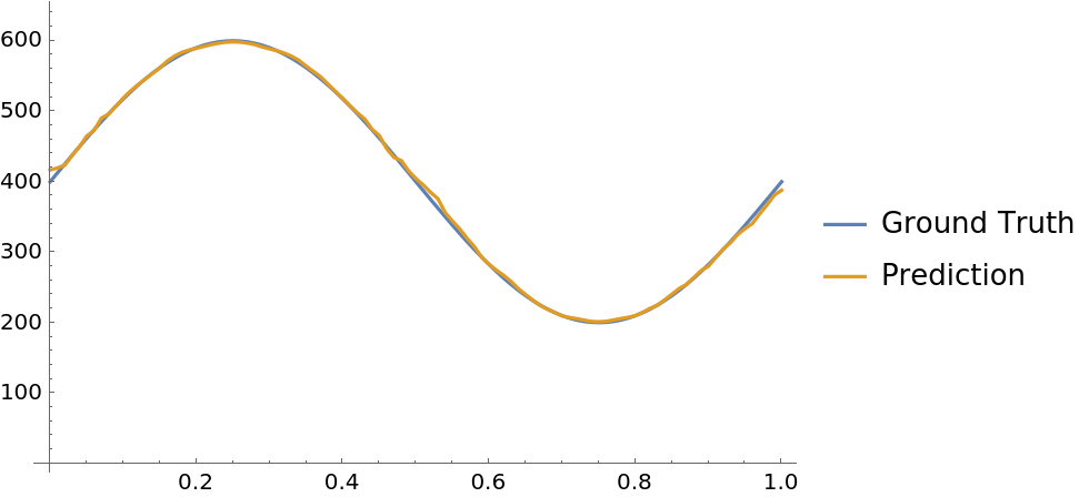
Compare the frequency predicted by the net with the ground truth:
Net information
Inspect the number of parameters of all arrays in the net:
Obtain the total number of parameters:
Obtain the layer type counts:
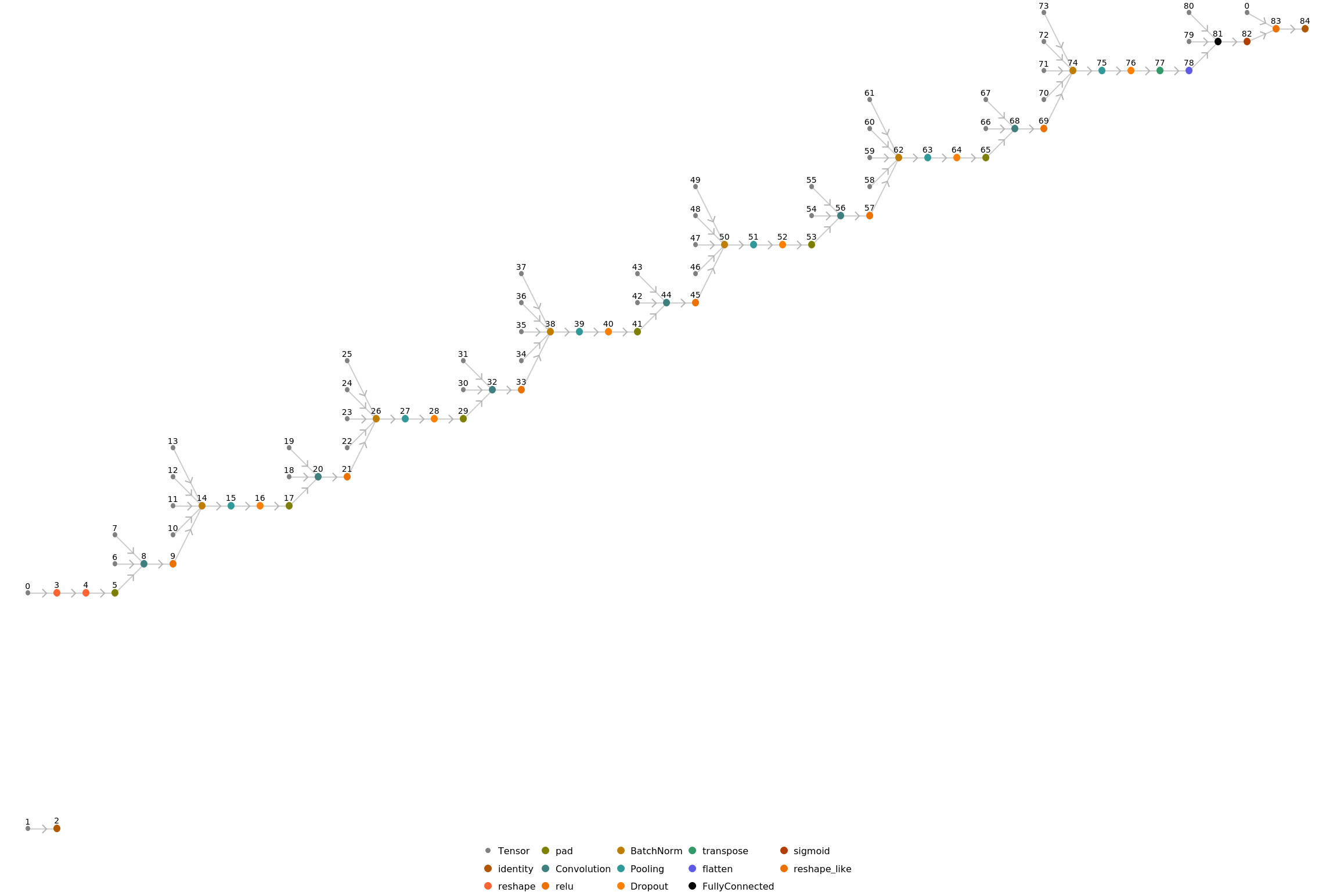
Display the summary graphic for the main net:
Export to MXNet
Export the net into a format that can be opened in MXNet:
Export also creates a net.params file containing parameters:
Get the size of the parameter file:
The size is similar to the byte count of the resource object:
Represent the MXNet net as a graph:
Resource History
Reference

![HMP = Module[
{starting, transition, emission, xx, yy, selfEmission}, starting = ConstantArray[1./360, 360];
yy = ConstantArray[Range[360], 360]; xx = Transpose@yy; transition = Map[Max[#, 0.] &, 12 - Abs[xx - yy], {2}]; transition = N@#/Total[#] & /@ transition; selfEmission = 0.1; emission = IdentityMatrix[360]*selfEmission + ConstantArray[(1. - selfEmission)/360., {360, 360}]; HiddenMarkovProcess[starting, transition, emission]
];](https://www.wolframcloud.com/obj/resourcesystem/images/f59/f59651b3-c8a0-453f-9a1a-8f63dc14c37c/60e490de25d7a77c.png)
![findPrediction["Interpolation", salience_, center_ : None] /; ArrayDepth[salience] == 2 := Map[Function[in, findPrediction["Interpolation", in, center]], salience]](https://www.wolframcloud.com/obj/resourcesystem/images/f59/f59651b3-c8a0-453f-9a1a-8f63dc14c37c/7e91998423285a9e.png)
![findPrediction["Interpolation", salience_, center_ : None] :=
Module[
{c, a, endpoints, cents},
If[center === None, c = First@Ordering[salience, -1], c = center];
endpoints = { Max[1, c - 4], Min[Length@salience, c + 5]}; a = Take[salience, endpoints];
cents = Range[0, 7180, 20] + 1997.3794084376191;
{10.*2^(Total[a*Take[cents, endpoints]]/Total[a] / 1200.), salience[[c]]}
]](https://www.wolframcloud.com/obj/resourcesystem/images/f59/f59651b3-c8a0-453f-9a1a-8f63dc14c37c/6bd9a7a610c02a23.png)
![findPrediction["Viterbi", salience_] := MapThread[
findPrediction["Interpolation", ##] &, {salience, FindHiddenMarkovStates[First[Ordering[#, -1]] & /@ salience, HMP]}]](https://www.wolframcloud.com/obj/resourcesystem/images/f59/f59651b3-c8a0-453f-9a1a-8f63dc14c37c/23c4b26d5a723c0f.png)
![netevaluation[a_?AudioQ, OptionsPattern[{"Decoder" -> "Viterbi"}]] := Module[
{res, times},
res = NetModel[
"CREPE Pitch Detection Net Trained on Monophonic Signal Data"][
AudioPad[a, {0.032, 0.032}]];
res = findPrediction[
OptionValue["Decoder"] /. Except["Viterbi"] -> "Interpolation", res];
times = {Range[0., QuantityMagnitude[Duration[a], "Seconds"], .01]};
<|"Prediction" -> TimeSeries[res[[All, 1]], times], "Confidence" -> TimeSeries[res[[All, 2]], times]|>
]](https://www.wolframcloud.com/obj/resourcesystem/images/f59/f59651b3-c8a0-453f-9a1a-8f63dc14c37c/063758486ac74753.png)
![ListLinePlot[pred["Prediction"], ColorFunction -> Function[{x, y}, Directive@Opacity@pred["Confidence"][x]], ColorFunctionScaling -> False, PlotRange -> {100, 120}]](https://www.wolframcloud.com/obj/resourcesystem/images/f59/f59651b3-c8a0-453f-9a1a-8f63dc14c37c/678a4d63a89b84af.png)
![ListLinePlot[<|"Ground Truth" -> Table[{t, f[t]}, {t, 0, 1, .01}], "Prediction" -> netevaluation[a]["Prediction"]|>]](https://www.wolframcloud.com/obj/resourcesystem/images/f59/f59651b3-c8a0-453f-9a1a-8f63dc14c37c/02643e44a39edbc5.png)
![NetInformation[
NetModel[
"CREPE Pitch Detection Net Trained on Monophonic Signal Data"], "ArraysElementCounts"]](https://www.wolframcloud.com/obj/resourcesystem/images/f59/f59651b3-c8a0-453f-9a1a-8f63dc14c37c/2c96ed6385a29e4b.png)

![NetInformation[
NetModel[
"CREPE Pitch Detection Net Trained on Monophonic Signal Data"], "ArraysTotalElementCount"]](https://www.wolframcloud.com/obj/resourcesystem/images/f59/f59651b3-c8a0-453f-9a1a-8f63dc14c37c/4bc4e3b254dd801c.png)
![NetInformation[
NetModel[
"CREPE Pitch Detection Net Trained on Monophonic Signal Data"], "LayerTypeCounts"]](https://www.wolframcloud.com/obj/resourcesystem/images/f59/f59651b3-c8a0-453f-9a1a-8f63dc14c37c/163429e30e90ed4c.png)
![NetInformation[
NetModel[
"CREPE Pitch Detection Net Trained on Monophonic Signal Data"][[
"Net"]], "SummaryGraphic"]](https://www.wolframcloud.com/obj/resourcesystem/images/f59/f59651b3-c8a0-453f-9a1a-8f63dc14c37c/3b6e7f8fb044fd62.png)
![jsonPath = Export[FileNameJoin[{$TemporaryDirectory, "net.json"}], NetModel[
"CREPE Pitch Detection Net Trained on Monophonic Signal Data"], "MXNet"]](https://www.wolframcloud.com/obj/resourcesystem/images/f59/f59651b3-c8a0-453f-9a1a-8f63dc14c37c/2bd3b5151285b146.png)