Resource retrieval
Get the pre-trained net:
NetModel parameters
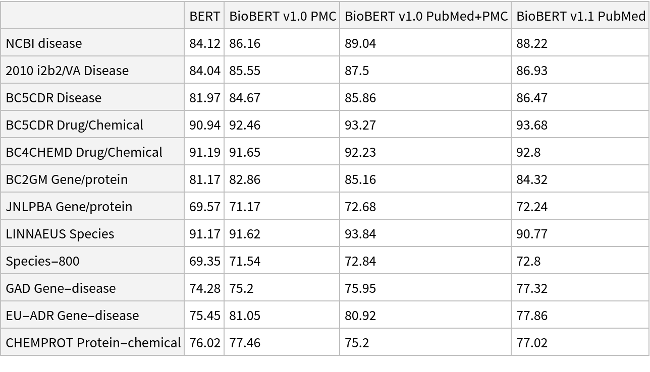
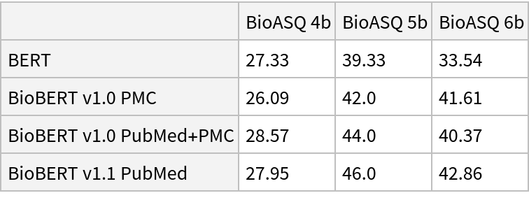
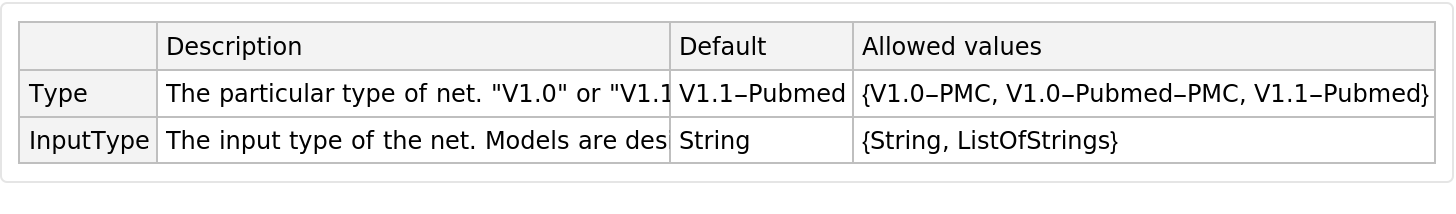
This model consists of a family of individual nets, each identified by a specific parameter combination. Inspect the available parameters:
Pick a non-default net by specifying the parameters:
Pick a non-default uninitialized net:
Basic usage
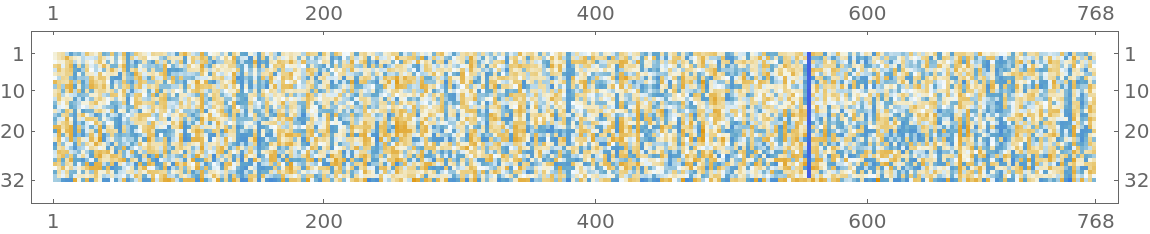
Given a piece of text, BioBERT net produces a sequence of feature vectors of size 768, which corresponds to the sequence of input words or subwords:
Obtain dimensions of the embeddings:
Visualize the embeddings:
Transformer architecture
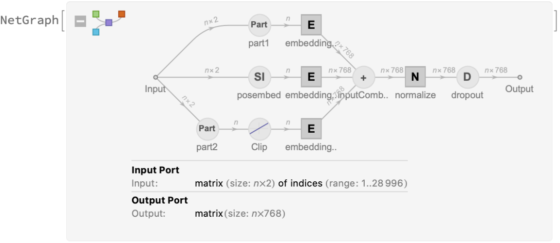
Each input text segment is first tokenized into words or subwords using a word-piece tokenizer and additional text normalization. Integer codes called token indices are generated from these tokens, together with additional segment indices:
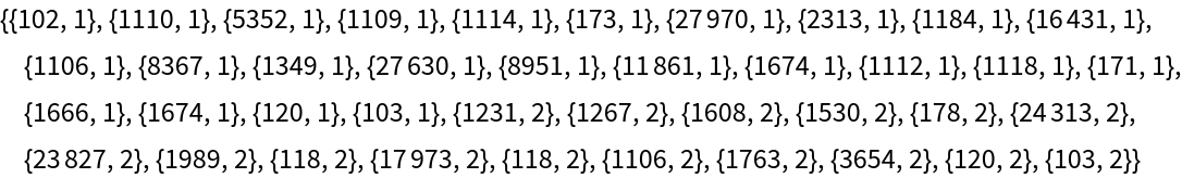
For each input subword token, the encoder yields a pair of indices that corresponds to the token index in the vocabulary and the index of the sentence within the list of input sentences:
The list of tokens always starts with special token index 102, which corresponds to the classification index.
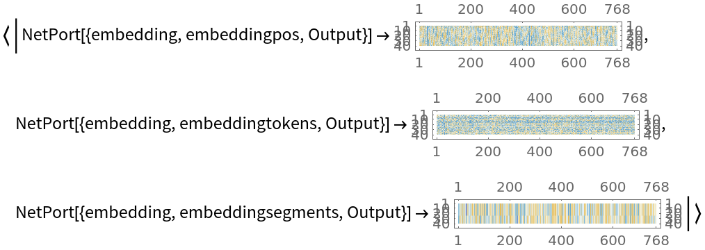
Also the special token index 103 is used as a separator between the different text segments. Each subword token is also assigned a positional index:
A lookup is done to map these indices to numeric vectors of size 768:
For each subword token, these three embeddings are combined by summing elements with ThreadingLayer:
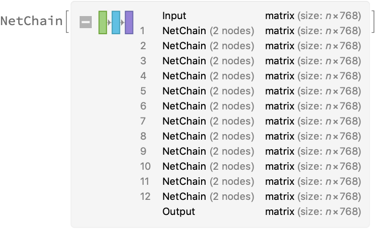
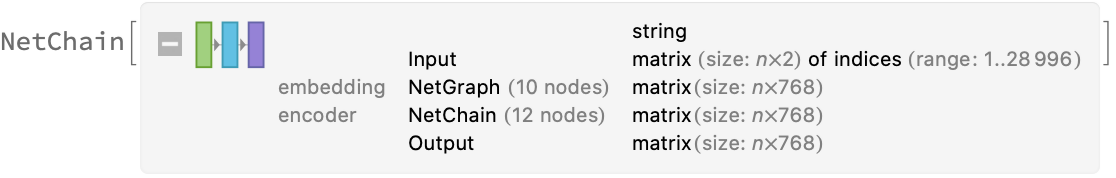
The transformer architecture then processes the vectors using 12 structurally identical self-attention blocks stacked in a chain:
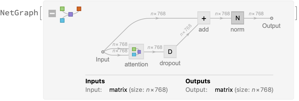
The key part of these blocks is the attention module comprising of 12 parallel self-attention transformations, also called “attention heads.” Each head uses an AttentionLayer at its core:
BioBERT uses self-attention, where the embedding of a given subword depends on the full input text. The following figure compares self-attention (lower left) to other types of connectivity patterns that are popular in deep learning:
Sentence analogies
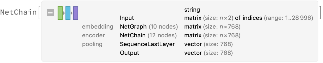
Define a sentence embedding net that takes the last feature vector from BioBERT subword embeddings (as an arbitrary choice):
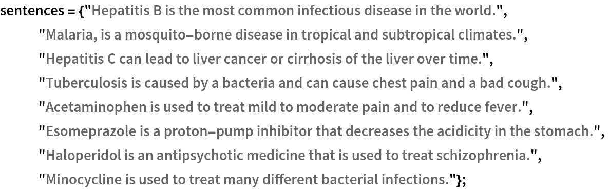
Define a list of sentences in two broad categories (food and music):
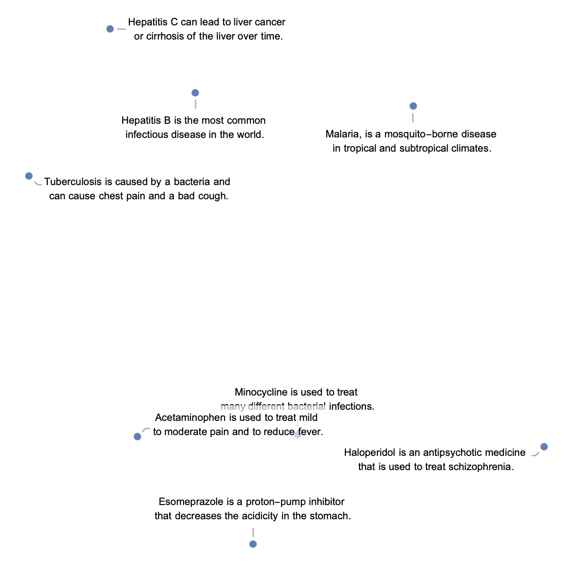
Precompute the embeddings for a list of sentences:
Visualize the similarity between the sentences using the net as a feature extractor:
Net information
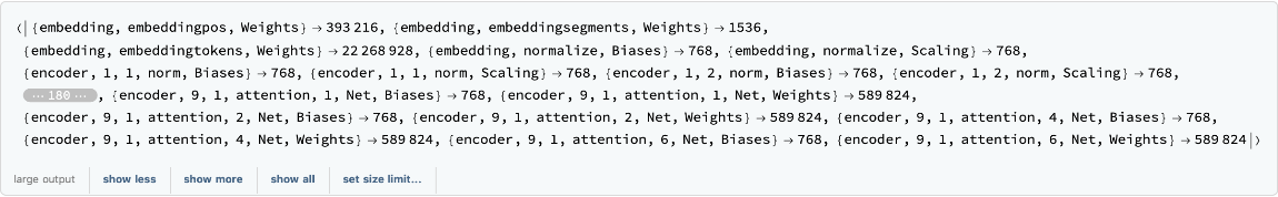
Inspect the number of parameters of all arrays in the net:
Obtain the total number of parameters:
Obtain the layer type counts:
Display the summary graphic:
Export to MXNet
Export the net into a format that can be opened in MXNet:
Export also creates a net.params file containing parameters:
Get the size of the parameter file:
![input = "Cushing syndrome symptoms with adrenal suppression is caused \
by a exogenous glucocorticoid depot triamcinolone.";
embeddings = NetModel["BioBERT Trained on PubMed and PMC Data"][input];](https://www.wolframcloud.com/obj/resourcesystem/images/40e/40e64897-0c45-4d74-bf9e-04e6139257f2/26e2acf52c611c2d.png)
![net[{"The patient was on clindamycin and topical tazarotene for his \
acne.", "His family history included hypertension, diabetes, and \
heart disease."}, NetPort[{"embedding", "posembed", "Output"}]]](https://www.wolframcloud.com/obj/resourcesystem/images/40e/40e64897-0c45-4d74-bf9e-04e6139257f2/195ef4606d2c8bbf.png)
![embeddings = net[{"The patient was on clindamycin and topical tazarotene for his \
acne.", "His family history included hypertension, diabetes, and \
heart disease."},
{NetPort[{"embedding", "embeddingpos", "Output"}],
NetPort[{"embedding", "embeddingtokens", "Output"}],
NetPort[{"embedding", "embeddingsegments", "Output"}]}];
Map[MatrixPlot, embeddings]](https://www.wolframcloud.com/obj/resourcesystem/images/40e/40e64897-0c45-4d74-bf9e-04e6139257f2/57d1b331bddee4ed.png)