Resource retrieval
Get the pre-trained net:
NetModel parameters
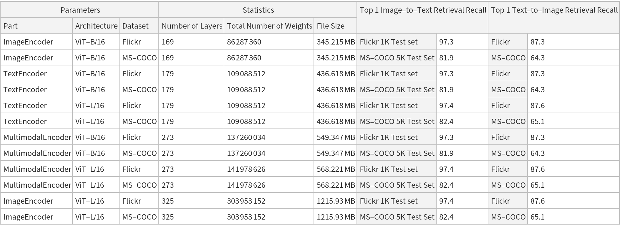
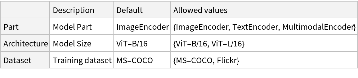
This model consists of a family of individual nets, each identified by a specific parameter combination. Inspect the available parameters:
Pick a non-default net by specifying the parameters:
Pick a non-default uninitialized net:
Basic usage
Define a test image:
Define a list of text descriptions:
Embed the test image and text descriptions into the same feature space:
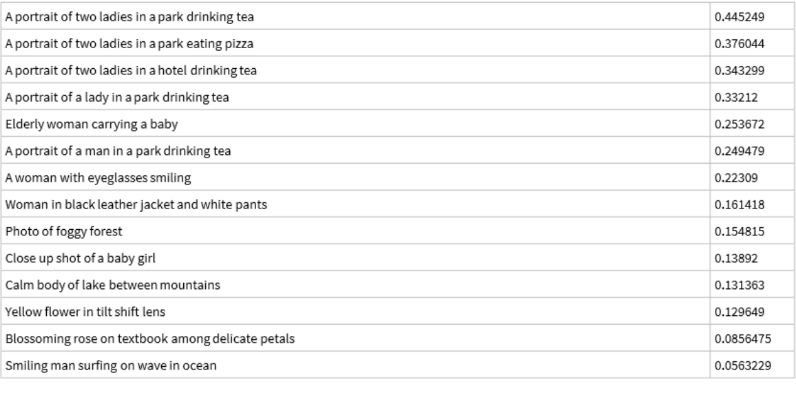
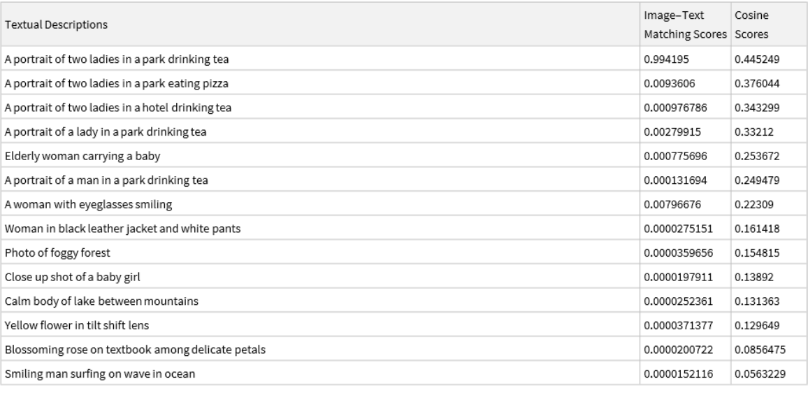
Rank the text description with respect to the correspondence to the input image according to the CosineDistance. Smaller distances (higher score) mean higher correspondence between the text and the image and higher cosine scores:
The "MultimodalEncoder" net outputs an image-text matching score that can be directly used to rank similarity between images and texts:
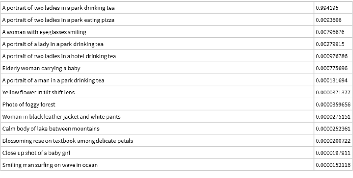
Rank the text description with respect to the correspondence to the input image according to the image-text matching score. Higher scores mean higher correspondence between the text and the image:
Note that the image-text matching scores are significantly more precise than the cosine similarity scores:
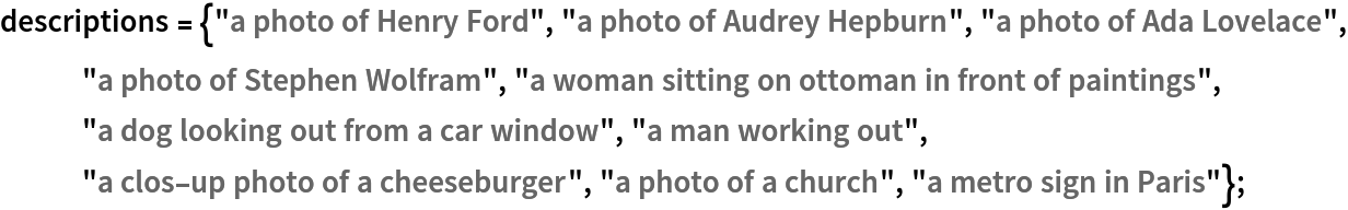
Compare a set of images with a set of texts using image-text matching scores:
Feature space visualization
Get a set of images:
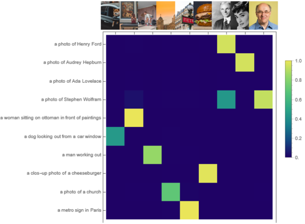
Visualize the feature space embedding performed by the image encoder. Notice that images from the same class are clustered together:
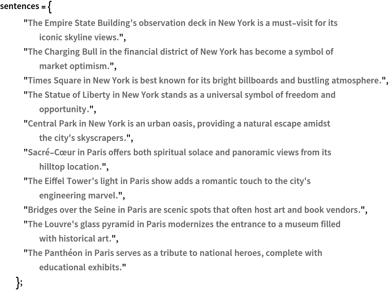
Define a list of sentences in two categories:
Visualize the similarity between the sentences using the net as a feature extractor:
Zero-shot image classification
By using the text and image feature extractors together, it's possible to perform generic image classification between any set of classes without having to explicitly train any model for those particular classes (zero-shot classification). Obtain the FashionMNIST test data, which contains ten thousand test images and 10 classes:
Display a few random examples from the set:
Get a mapping between class IDs and labels:
Generate the text templates for the FashionMNIST labels and embed them. The text templates will effectively act as classification labels:
Classify an image from the test set. Obtain its embedding:
The result of the classification is the description that has the highest similarity score:
Find the top 10 descriptions closest to the image:
Cross-attention visualization for images
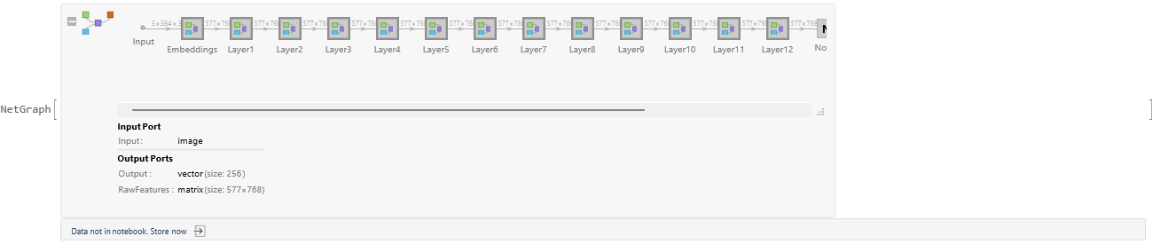
When processing its image and text inputs, the multimodal encoder attends on the image features produced by the image encoder. Such features are a set of 577 vectors of length 768, where every vector except the first one corresponds to one of 24x24 patches taken from the input image (the extra vector exists because the image encoder inherits the architecture of the image classification model Vision Transformer Trained on ImageNet Competition Data, but in this case, it doesn't have any special importance). This means that the multimodal encoder's attention weights to these image features can be interpreted as the image patches the encoder is "looking at" for every token of the input text, and it is possible to visualize this information. Get a test image and compute the features:
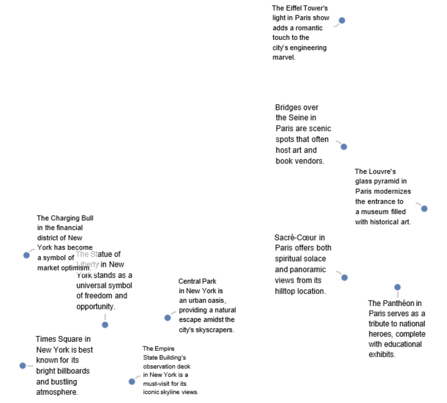
Feed the feature and some text to the multimodal encoder. There are 12 attention blocks in the encoder and each generates its own set of attention weights. Inspect the attention weights for a single block:
Each token corresponds to a 12x577 array of attention weights, where 12 is the number of the attention heads and 577 is the 24x24 patches plus the extra one:
Extract the attention weights related to the image patches:
Reshape the flat image patch dimension to 24x24 and take the average over the attention heads, thus obtaining a 24x24 attention matrix for each token:
To reveal novel patch interactions specific to each token, suppress the consistently high attention weights by subtracting the minimum value aggregated across the token dimension:
Visualize the attention weight matrices. Patches with higher values (red) are what is mostly being "looked at" when generating the corresponding token:
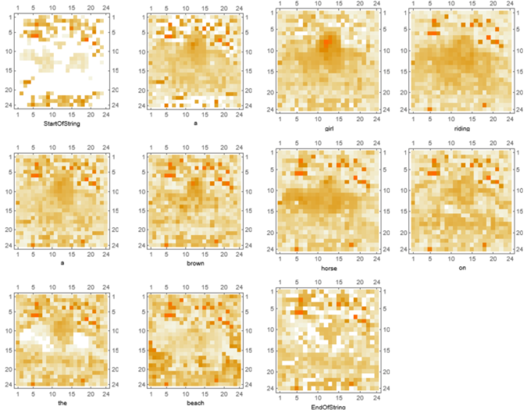
Define a function to visualize the attention matrix on the image:
Visualize the attention mechanism for each token. A recurrent noisy pattern of large positive activation can be observed, but notice the emphasis on the girl for the token "girl" and the beach for the token "beach":
Net information
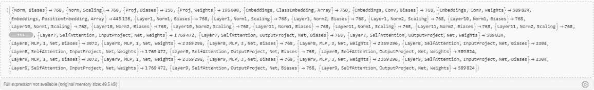
Inspect the number of parameters of all arrays in the net:
Obtain the total number of parameters:
Obtain the layer type counts:
![NetModel["BLIP Image-Text Matching Nets Trained on Captioning Datasets", "ParametersInformation"]](https://www.wolframcloud.com/obj/resourcesystem/images/6db/6dbeb429-17ce-43ed-a925-2c6d84fe51d1/7b70704511bc9f7b.png)
![NetModel[{"BLIP Image-Text Matching Nets Trained on Captioning Datasets", "Part" -> "MultimodalEncoder", "Architecture" -> "ViT-L/16"}]](https://www.wolframcloud.com/obj/resourcesystem/images/6db/6dbeb429-17ce-43ed-a925-2c6d84fe51d1/4e1c1e881ca3f15f.png)
![NetModel[{"BLIP Image-Text Matching Nets Trained on Captioning Datasets", "Part" -> "TextEncoder"}, "UninitializedEvaluationNet"]](https://www.wolframcloud.com/obj/resourcesystem/images/6db/6dbeb429-17ce-43ed-a925-2c6d84fe51d1/7bb6a7c8a79360da.png)
![(* Evaluate this cell to get the example input *) CloudGet["https://www.wolframcloud.com/obj/1b9f7ff2-1f1b-46b3-8f7d-1106d55d5a31"]](https://www.wolframcloud.com/obj/resourcesystem/images/6db/6dbeb429-17ce-43ed-a925-2c6d84fe51d1/16ab76fc43de4fc6.png)
![{textEncoder, imageEncoder} = NetModel[{"BLIP Image-Text Matching Nets Trained on Captioning Datasets", "Part" -> #}] & /@ {"TextEncoder", "ImageEncoder"};](https://www.wolframcloud.com/obj/resourcesystem/images/6db/6dbeb429-17ce-43ed-a925-2c6d84fe51d1/768e8df0720f1ffa.png)
![multimodalEncoder = NetModel[{"BLIP Image-Text Matching Nets Trained on Captioning Datasets", "Part" -> "MultimodalEncoder"}];](https://www.wolframcloud.com/obj/resourcesystem/images/6db/6dbeb429-17ce-43ed-a925-2c6d84fe51d1/107751c008cd1685.png)
![itmScores = multimodalEncoder[<|"Input" -> descriptions, "ImageFeatures" -> ConstantArray[imgFeatures, Length[descriptions]]|>];](https://www.wolframcloud.com/obj/resourcesystem/images/6db/6dbeb429-17ce-43ed-a925-2c6d84fe51d1/570ded7fad8a39f0.png)
![ReverseSortBy[
Transpose@
Dataset[<|"Textual Descriptions" -> descriptions, "Image-Text \nMatching Scores" -> itmScores[[;; , 2]], "Cosine\nScores" -> cosineScores|>], Last]](https://www.wolframcloud.com/obj/resourcesystem/images/6db/6dbeb429-17ce-43ed-a925-2c6d84fe51d1/4e2343864c568d38.png)
![(* Evaluate this cell to get the example input *) CloudGet["https://www.wolframcloud.com/obj/9638e54d-4e0a-48e9-bb29-bcebf800fb62"]](https://www.wolframcloud.com/obj/resourcesystem/images/6db/6dbeb429-17ce-43ed-a925-2c6d84fe51d1/1a08570396836510.png)
![ArrayPlot[
itmScores,
ColorFunction -> "BlueGreenYellow",
PlotLegends -> Automatic,
FrameTicks -> {
{Transpose[{Range[Length[descriptions]], descriptions}], None}, {None, Transpose[{Range[Length[images]], ImageResize[#, 60] & /@ images}]}
}
, ImageSize -> Large
]](https://www.wolframcloud.com/obj/resourcesystem/images/6db/6dbeb429-17ce-43ed-a925-2c6d84fe51d1/27c00f5ae7d5bdf7.png)
![(* Evaluate this cell to get the example input *) CloudGet["https://www.wolframcloud.com/obj/b9826de5-68db-4583-ba36-d8aacb6240d1"]](https://www.wolframcloud.com/obj/resourcesystem/images/6db/6dbeb429-17ce-43ed-a925-2c6d84fe51d1/3a20ba2e6c741b1b.png)
![FeatureSpacePlot[
Thread[NetModel[{"BLIP Image-Text Matching Nets Trained on Captioning Datasets", "Part" -> "ImageEncoder"}][imgs, NetPort[{"Proj", "Output"}]] -> imgs],
LabelingSize -> 70,
RandomSeeding -> 37,
LabelingFunction -> Callout,
ImageSize -> 700,
AspectRatio -> 0.9
]](https://www.wolframcloud.com/obj/resourcesystem/images/6db/6dbeb429-17ce-43ed-a925-2c6d84fe51d1/5ca5fe46e5b5364a.png)
![FeatureSpacePlot[
Thread[NetModel[{"BLIP Image-Text Matching Nets Trained on Captioning Datasets", "Part" -> "TextEncoder"}][
sentences] -> (Tooltip[Style[Text@#, Medium]] & /@ sentences)],
LabelingSize -> {100, 100},
RandomSeeding -> 37,
LabelingFunction -> Callout,
ImageSize -> 700,
AspectRatio -> 0.9
]](https://www.wolframcloud.com/obj/resourcesystem/images/6db/6dbeb429-17ce-43ed-a925-2c6d84fe51d1/70d40ea6e8482539.png)

![imgFeatures = NetModel[{"BLIP Image-Text Matching Nets Trained on Captioning Datasets", "Part" -> "ImageEncoder"}][img, NetPort["RawFeatures"]];](https://www.wolframcloud.com/obj/resourcesystem/images/6db/6dbeb429-17ce-43ed-a925-2c6d84fe51d1/3b6265d717d9abff.png)
![scores = NetModel[{"BLIP Image-Text Matching Nets Trained on Captioning Datasets", "Part" -> "MultimodalEncoder"}][<|
"Input" -> labelTemplates, "ImageFeatures" -> ConstantArray[imgFeatures, Length[labelTemplates]]|>];](https://www.wolframcloud.com/obj/resourcesystem/images/6db/6dbeb429-17ce-43ed-a925-2c6d84fe51d1/30a699a33d59b2ac.png)

![(* Evaluate this cell to get the example input *) CloudGet["https://www.wolframcloud.com/obj/19b223e8-ec43-4586-b11d-cf42ce05642f"]](https://www.wolframcloud.com/obj/resourcesystem/images/6db/6dbeb429-17ce-43ed-a925-2c6d84fe51d1/0f62f68168563bc7.png)
![imgFeatures = NetModel[{"BLIP Image-Text Matching Nets Trained on Captioning Datasets", "Part" -> "ImageEncoder"}][testImage, NetPort["RawFeatures"]];](https://www.wolframcloud.com/obj/resourcesystem/images/6db/6dbeb429-17ce-43ed-a925-2c6d84fe51d1/4a486fb3b2a3b05e.png)
![description = "a girl riding a brown horse on the beach";
tokenizer = NetExtract[
NetModel[{"BLIP Image-Text Matching Nets Trained on Captioning Datasets", "Part" -> "TextEncoder"}], "Input"];
allTokens = NetExtract[tokenizer, "Tokens"];
codes = tokenizer[description];
tokens = allTokens[[codes]];](https://www.wolframcloud.com/obj/resourcesystem/images/6db/6dbeb429-17ce-43ed-a925-2c6d84fe51d1/0c778e7ca6b20956.png)
![tokenAttentionWeights = Thread[tokens -> NetModel[{"BLIP Image-Text Matching Nets Trained on Captioning Datasets", "Part" -> "MultimodalEncoder"}][<|"Input" -> description, "ImageFeatures" -> imgFeatures|>, NetPort[{"TextEncoder", "TextLayer1", "CrossAttention", "Attention", "AttentionWeights"}]]];](https://www.wolframcloud.com/obj/resourcesystem/images/6db/6dbeb429-17ce-43ed-a925-2c6d84fe51d1/17d1f52f59611ac0.png)
![attentionWeights = ArrayReshape[
attentionWeights, {numTokens, numHeads, Sqrt[numPatches], Sqrt[numPatches]}];
attentionWeights = Map[Mean, attentionWeights, {1}];
attentionWeights // Dimensions](https://www.wolframcloud.com/obj/resourcesystem/images/6db/6dbeb429-17ce-43ed-a925-2c6d84fe51d1/1298d48372dfdeb4.png)
![GraphicsGrid[
Partition[
MapThread[
Labeled[#1, #2] &, {MatrixPlot /@ attentionWeights, Keys[tokenAttentionWeights]}], 4, 4, {1, 1}, ""], ImageSize -> Large]](https://www.wolframcloud.com/obj/resourcesystem/images/6db/6dbeb429-17ce-43ed-a925-2c6d84fe51d1/5bd1a3036be5eb89.png)
![visualizeAttention[img_Image, attentionMatrix_, label_] := Block[{heatmap, wh},
wh = ImageDimensions[img];
heatmap = ImageApply[{#, 1 - #, 1 - #} &, ImageAdjust@Image[attentionMatrix]];
heatmap = ImageResize[heatmap, ImageDimensions[img]];
Labeled[ImageCompose[img, {ColorConvert[heatmap, "RGB"], 0.5}], label]
]](https://www.wolframcloud.com/obj/resourcesystem/images/6db/6dbeb429-17ce-43ed-a925-2c6d84fe51d1/7231fdef4ba3e803.png)
![Information[
NetModel[
"BLIP Image-Text Matching Nets Trained on Captioning Datasets"], "ArraysElementCounts"]](https://www.wolframcloud.com/obj/resourcesystem/images/6db/6dbeb429-17ce-43ed-a925-2c6d84fe51d1/536c01a8f80eb7e1.png)
![Information[
NetModel[
"BLIP Image-Text Matching Nets Trained on Captioning Datasets"], "ArraysTotalElementCount"]](https://www.wolframcloud.com/obj/resourcesystem/images/6db/6dbeb429-17ce-43ed-a925-2c6d84fe51d1/63a8a3c7ae320d04.png)
![Information[
NetModel[
"BLIP Image-Text Matching Nets Trained on Captioning Datasets"], "LayerTypeCounts"]](https://www.wolframcloud.com/obj/resourcesystem/images/6db/6dbeb429-17ce-43ed-a925-2c6d84fe51d1/093f158335009ab5.png)
