Resource retrieval
Get the pre-trained net:
NetModel parameters
This model consists of a family of individual nets, each identified by a specific parameter combination. Inspect the available parameters:
Pick a non-default net by specifying the parameters:
Pick a non-default uninitialized net:
Evaluation function
Write an evaluation function to scale the result to the input image size and suppress the least probable detections:
Basic usage
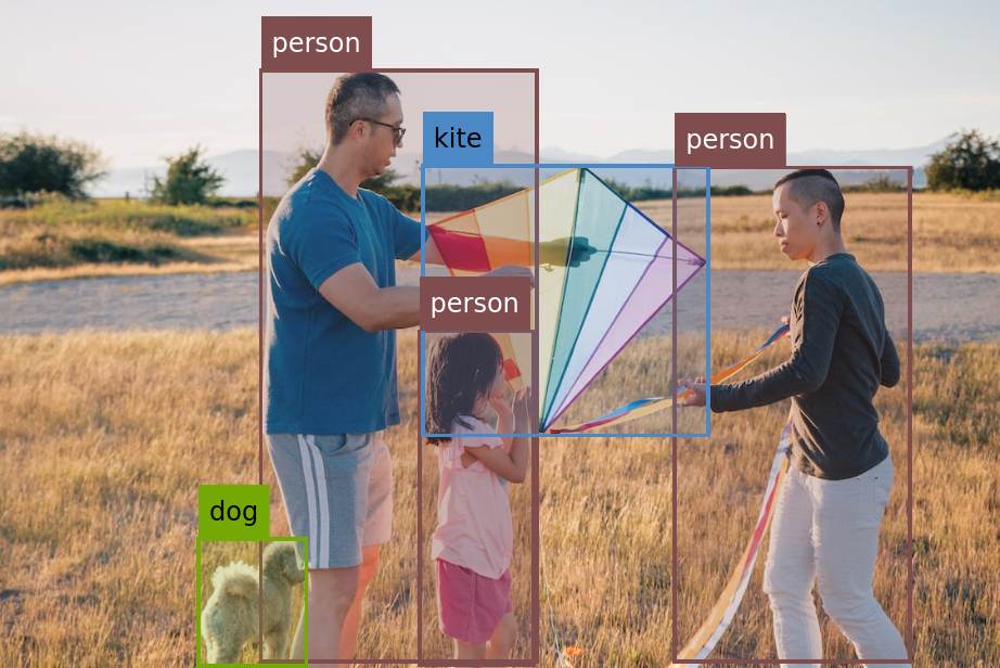
Obtain the detected bounding boxes with their corresponding classes and confidences for a given image:
The model's output is an Association containing the detected "Boxes", "Classes" and "Masks":
The "Boxes" key is a list of Rectangle expressions corresponding to the bounding boxes of the detected objects:
The "Classes" key contains the classes of the detected objects:
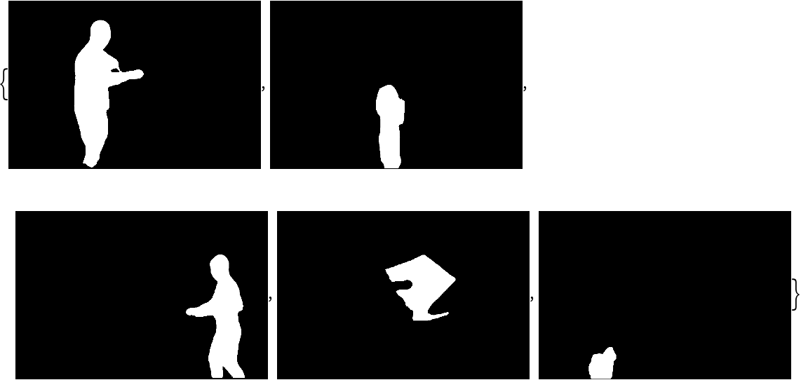
The "Masks" key contains segmentation masks for the detected objects:
Visualize the boxes labeled with their assigned classes:
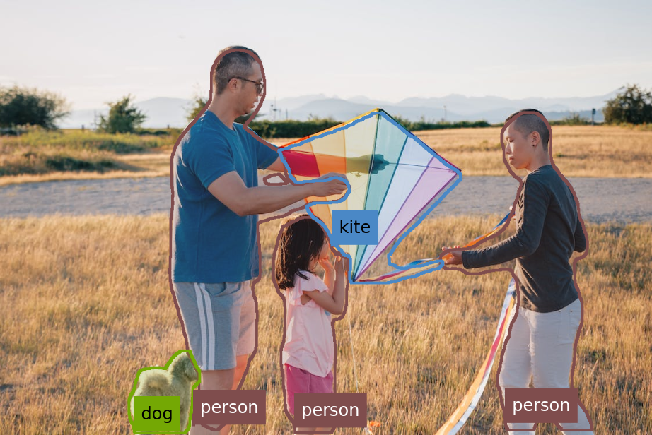
Visualize the masks labeled with their assigned classes:
Network result
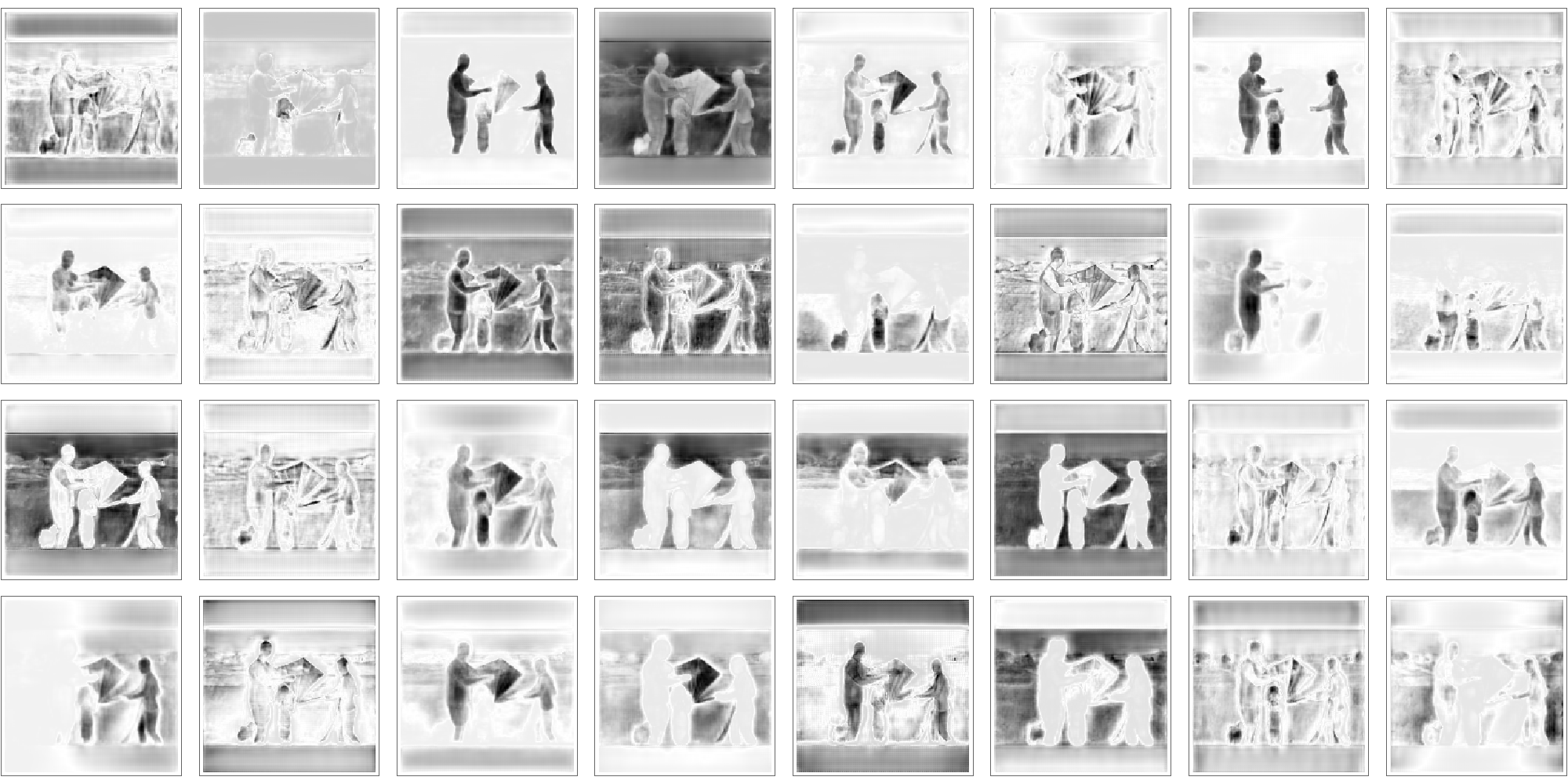
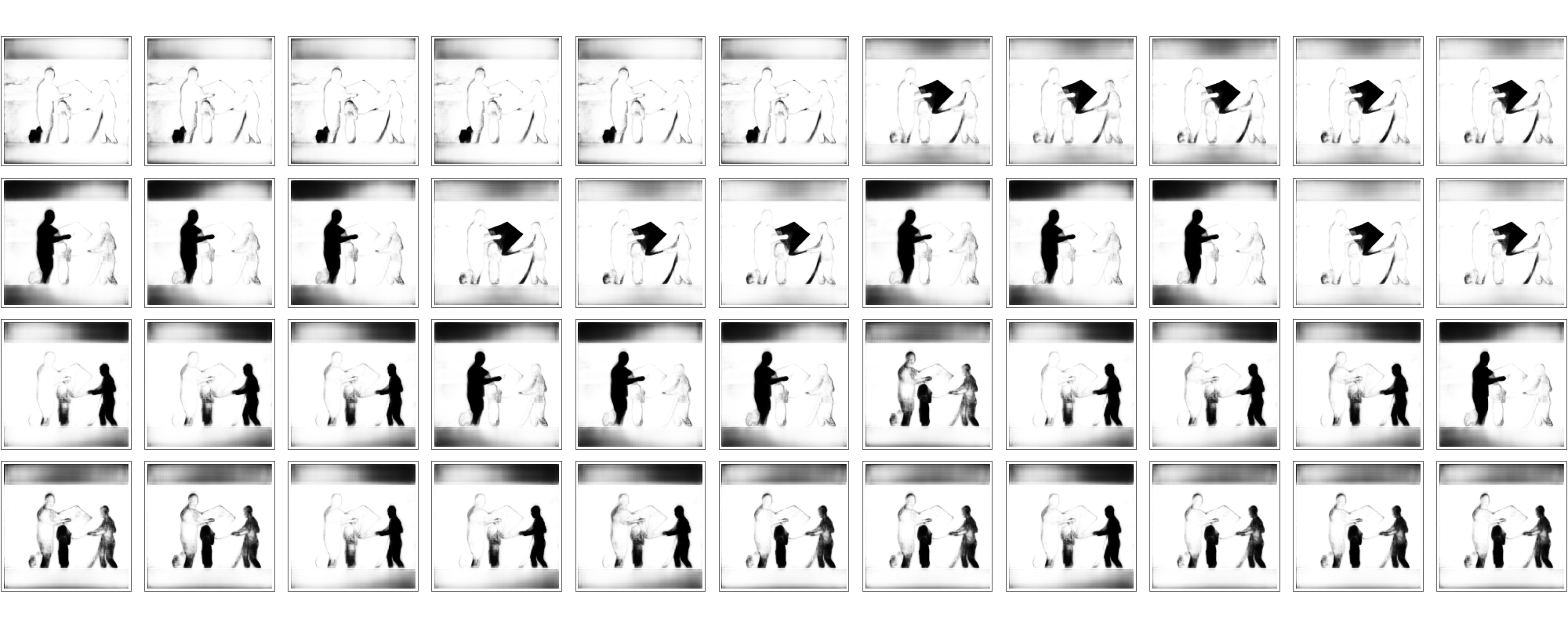
The network computes eight thousand four hundred bounding boxes, the probability that the objects in each box are of any given class, 32 160x160 prototyped segmentation masks and mask weights for each bounding box:
Visualize prototyped masks:
Every box is then assigned a mask, computed by taking linear combinations of the prototyped masks with the associated weights. Values are normalized to lie between 0 and 1 with a LogisticSigmoid:
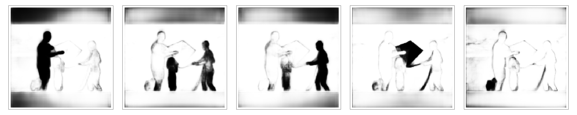
Filter out masks whose detection probabilities are small and visualize the others:
Scale the boxes and apply non-maximum suppression for the final reduction. Use the result to filter the masks and visualize them:
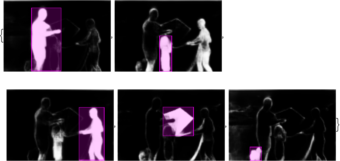
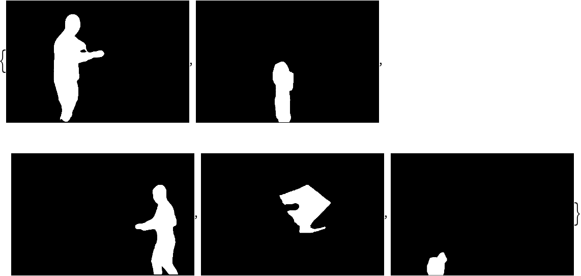
Remove the padding from the masks, scale them to the original image size, binarize them and use the scaled boxes to isolate the region of interest:
Remove any detections outside the boxes:
Visualize the bounding boxes scaled by their class probabilities:
Visualize all the boxes scaled by the probability that they contain a person:
Superimpose the person predictions on top of the input received by the net:
Net information
Inspect the number of parameters of all arrays in the net:
Obtain the total number of parameters:
Obtain the layer type counts:
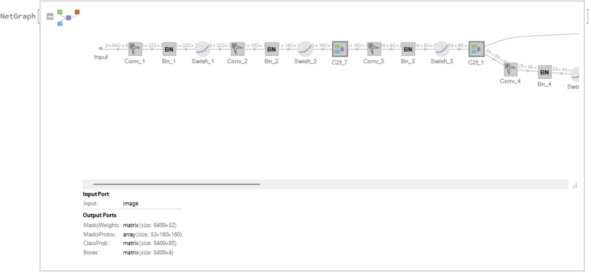
Display the summary graphic:
![NetModel[{"YOLO V8 Segment Trained on MS-COCO Data", "Size" -> "L"}, "UninitializedEvaluationNet"]](https://www.wolframcloud.com/obj/resourcesystem/images/6cf/6cfe148d-2d2e-4541-9a83-0b806dd60b48/5e975b9212aa7b5f.png)
![(* Evaluate this cell to get the example input *) CloudGet["https://www.wolframcloud.com/obj/d8f9c7a2-8d27-4346-8fe4-da28a08c83a2"]](https://www.wolframcloud.com/obj/resourcesystem/images/6cf/6cfe148d-2d2e-4541-9a83-0b806dd60b48/25e6f2e0d168289b.png)
![(* Evaluate this cell to get the example input *) CloudGet["https://www.wolframcloud.com/obj/2dff7112-edaf-4981-9801-4a254b705432"]](https://www.wolframcloud.com/obj/resourcesystem/images/6cf/6cfe148d-2d2e-4541-9a83-0b806dd60b48/58d37a64545b6f9f.png)
![isDetection = UnitStep[Max /@ res["ClassProb"] - 0.45];
probableMasks = Pick[masks, isDetection, 1];
GraphicsGrid[Partition[Map[ArrayPlot, probableMasks], 11], ImageSize -> {1000, 400}]](https://www.wolframcloud.com/obj/resourcesystem/images/6cf/6cfe148d-2d2e-4541-9a83-0b806dd60b48/416322574f55196c.png)
![{probableClasses, probableBoxes} = Map[Pick[#, isDetection, 1] &, {res["ClassProb"], res["Boxes"]}];
{w, h} = ImageDimensions[testImage];
imgSize = 640;
max = Max[{w, h}];
scale = max/imgSize;
{padx, pady} = imgSize*(1 - {w, h}/max)/2;
{probableRectangles, probableBoxes} =
Transpose@Apply[
Function[
x1 = Clip[Floor[scale*(#1 - #3/2 - padx)], {1, w}];
y1 = Clip[Floor[scale*(imgSize - #2 - #4/2 - pady)], {1, h}];
x2 = Clip[Floor[scale*(#1 + #3/2 - padx)], {1, w}];
y2 = Clip[Floor[scale*(imgSize - #2 + #4/2 - pady)], {1, h}];
{
Rectangle[{x1, y1}, {x2, y2}],
{{x1, Clip[Floor[scale*(#2 - #4/2 - pady)], {1, h}]}, {x2, Clip[Floor[scale*(#2 + #4/2 - pady)], {1, h}]}}
}
],
probableBoxes,
2
];
nms = ResourceFunction["NonMaximumSuppression"][
probableRectangles -> Max /@ probableClasses, "Index", MaxOverlapFraction -> 0.45];
nmsMasks = probableMasks[[nms]];
GraphicsRow[Map[ArrayPlot, nmsMasks], ImageSize -> {1000, 200}]](https://www.wolframcloud.com/obj/resourcesystem/images/6cf/6cfe148d-2d2e-4541-9a83-0b806dd60b48/0b04352b63e5da86.png)
![nmsRectangles = probableRectangles[[nms]];
{w, h} = ImageDimensions[testImage];
{mh, mw} = {160, 160};
gain = Min[{mh, mw}/{w, h}];
pad = ({mw, mh} - {w, h}*gain)/2;
{left, top} = Clip[Floor[pad], {1, mh}];
{right, bottom} = Clip[Floor[{mw, mh} - pad], {1, mh}];
croppedMasks = nmsMasks[[All, top ;; bottom, left ;; right]];
resampledMasks = ArrayResample[croppedMasks, {Length[croppedMasks], h, w}, Resampling -> "Linear"];
MapThread[
HighlightImage[
Image[#1, Interleaving -> False], #2] &, {resampledMasks, nmsRectangles}]](https://www.wolframcloud.com/obj/resourcesystem/images/6cf/6cfe148d-2d2e-4541-9a83-0b806dd60b48/6f4b9a78e1665a8d.png)
![nmsBoxes = Part[probableBoxes, nms];
binarizedMasks = MapThread[(
mask = ConstantArray[0, Dimensions[#1]];
imask = Take[#1, #2[[1, 2]] ;; #2[[2, 2]], #2[[1, 1]] ;; #2[[2, 1]]];
mask[[#2[[1, 2]] ;; #2[[2, 2]], #2[[1, 1]] ;; #2[[2, 1]]]] = imask;
Binarize[Image[mask, Interleaving -> False], 0.5]) &,
{resampledMasks, nmsBoxes}
]](https://www.wolframcloud.com/obj/resourcesystem/images/6cf/6cfe148d-2d2e-4541-9a83-0b806dd60b48/3aa590fdc17ea411.png)
![{w, h} = ImageDimensions[testImage];
imgSize = 640;
max = Max[{w, h}];
scale = max/imgSize;
{padx, pady} = imgSize*(1 - {w, h}/max)/2;
rectangles = Apply[
Function[
x1 = Clip[Floor[scale*(#1 - #3/2 - padx)], {1, w}];
y1 = Clip[Floor[scale*(imgSize - #2 - #4/2 - pady)], {1, h}];
x2 = Clip[Floor[scale*(#1 + #3/2 - padx)], {1, w}];
y2 = Clip[Floor[scale*(imgSize - #2 + #4/2 - pady)], {1, h}];
Rectangle[{x1, y1}, {x2, y2}]
],
res["Boxes"],
2
];
Graphics[
MapThread[
{EdgeForm[Opacity[Total[#1] + .01]], #2} &, {Max /@ res["ClassProb"], rectangles}],
BaseStyle -> {FaceForm[], EdgeForm[{Thin, Black}]}
]](https://www.wolframcloud.com/obj/resourcesystem/images/6cf/6cfe148d-2d2e-4541-9a83-0b806dd60b48/15261d6091bdd6c5.png)

![Graphics[
MapThread[{EdgeForm[Opacity[#1 + .01]], #2} &, {Extract[
res["ClassProb"], {All, idx}], rectangles}],
BaseStyle -> {FaceForm[], EdgeForm[{Thin, Black}]}
]](https://www.wolframcloud.com/obj/resourcesystem/images/6cf/6cfe148d-2d2e-4541-9a83-0b806dd60b48/42ad3433c9f14000.png)

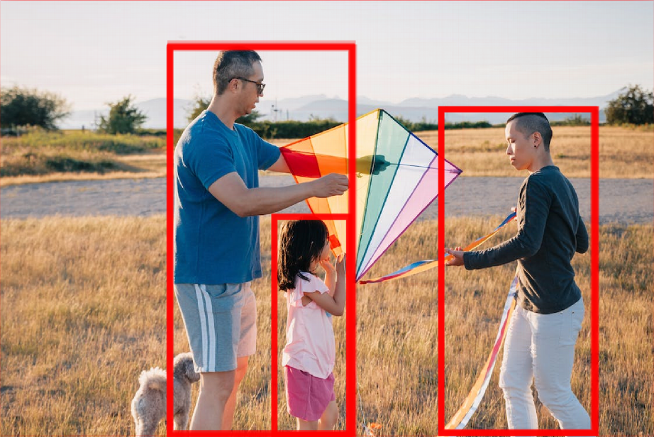
![HighlightImage[testImage, Graphics[
MapThread[{EdgeForm[{Thickness[#1/100], Opacity[(#1 + .01)/3]}], #2} &, {Extract[
res["ClassProb"], {All, idx}], rectangles}]], BaseStyle -> {FaceForm[], EdgeForm[{Thin, Red}]}]](https://www.wolframcloud.com/obj/resourcesystem/images/6cf/6cfe148d-2d2e-4541-9a83-0b806dd60b48/3f9f706fb01dca8e.png)
![Information[
NetModel[
"YOLO V8 Segment Trained on MS-COCO Data"], "ArraysTotalElementCount"]](https://www.wolframcloud.com/obj/resourcesystem/images/6cf/6cfe148d-2d2e-4541-9a83-0b806dd60b48/395bf62d8028cf5f.png)

