Resource retrieval
Get the pre-trained net:
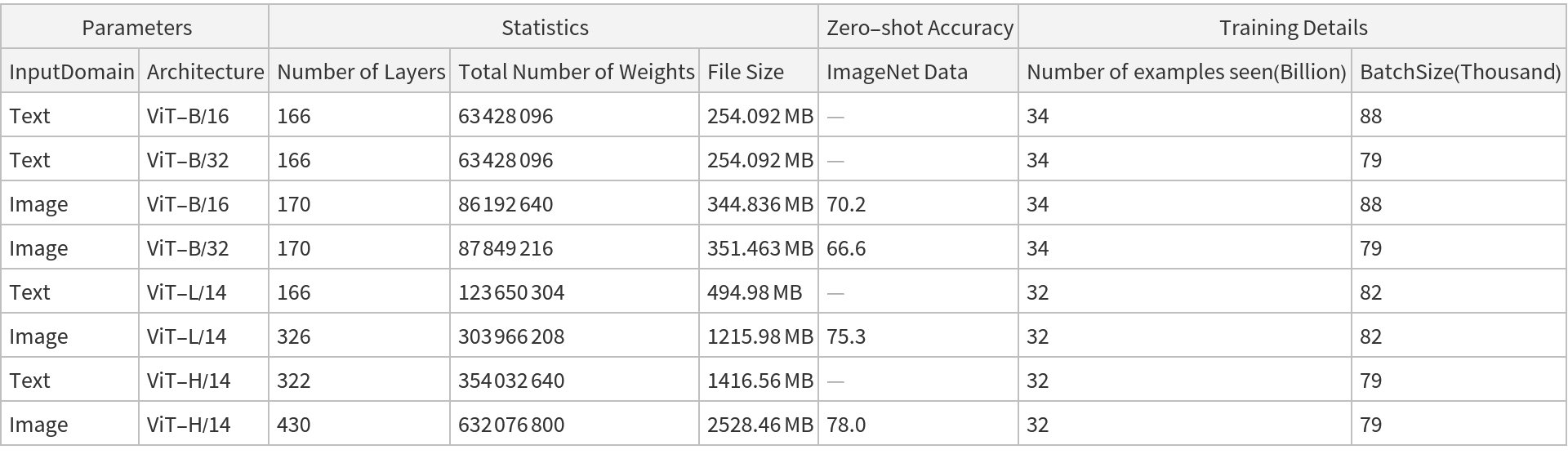
NetModel parameters
This model consists of a family of individual nets, each identified by a specific parameter combination. Inspect the available parameters:
Pick a non-default net by specifying the parameters:
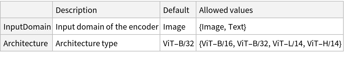
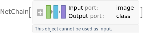
Pick a non-default uninitialized net:
Basic usage
Use the OpenCLIP text encoder to obtain the feature representation of a piece of text:
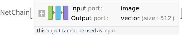
The default OpenCLIP text encoder embeds the input text into a vector of size 512:
Use the OpenCLIP image encoder to obtain the feature representation of an image:
The default OpenCLIP image encoder embeds the input text into a vector of size 512:
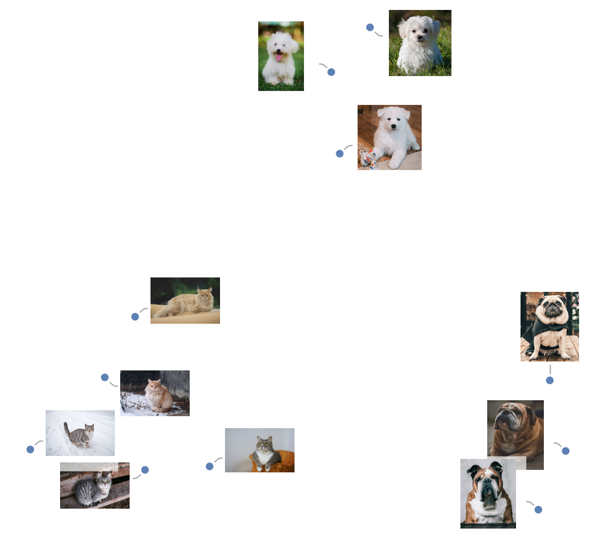
Feature space visualization
Get a set of images:
Visualize the features of a set of images:
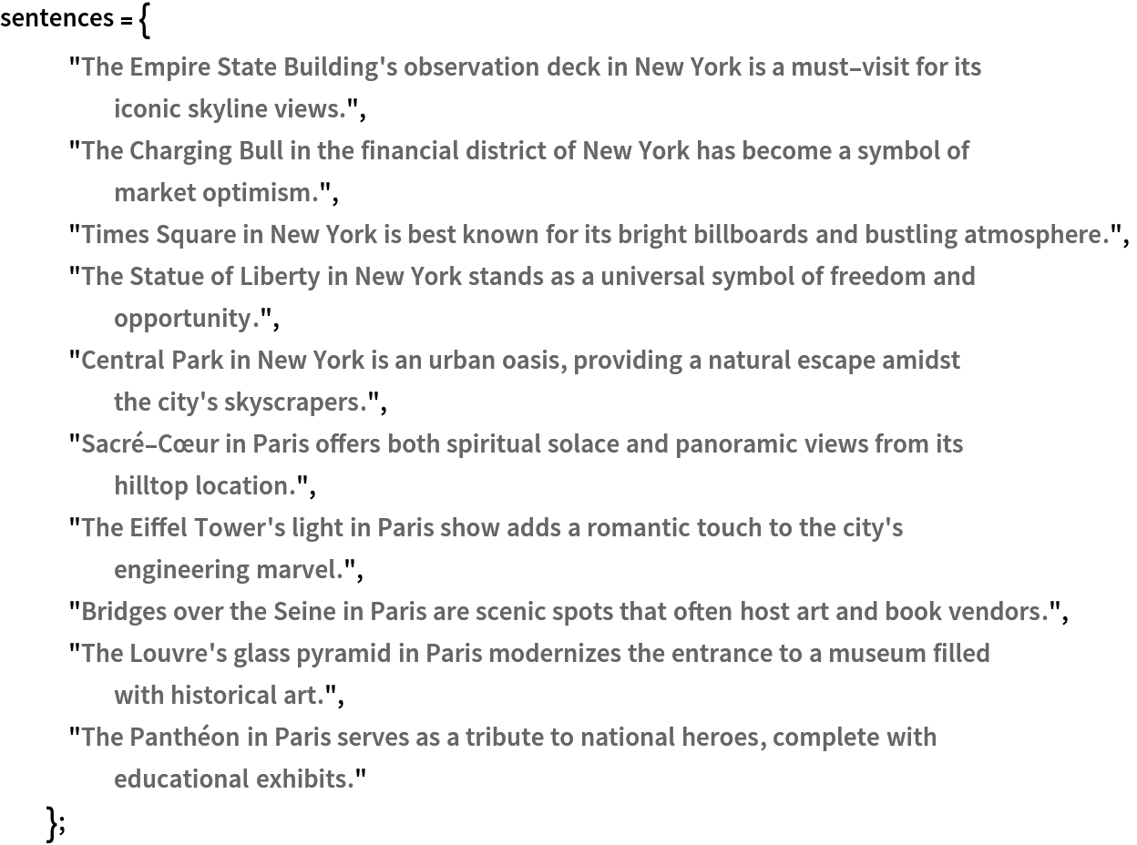
Define a list of sentences in two broad categories:
Visualize the similarity between the sentences using the net as a feature extractor:
Connecting text and images
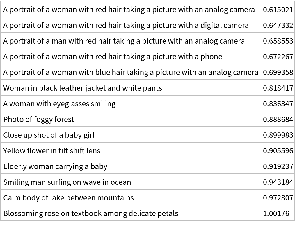
Define a test image:
Define a list of text descriptions:
Embed the test image and text descriptions into the same feature space:
Rank the text description with respect to the correspondence to the input image according to the CosineDistance. Smaller distances mean higher correspondence between the text and the image:
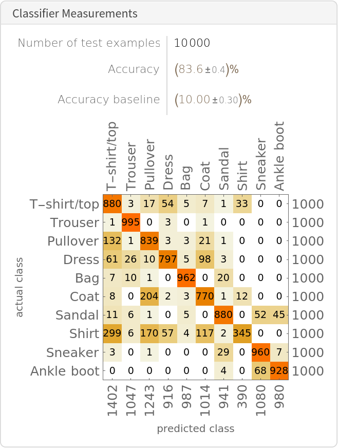
Zero-shot image classification
By using the text and image feature extractors together, it's possible to perform generic image classification between any set of classes without having to explicitly train any model for those particular classes (zero-shot classification). Obtain the FashionMNIST test data, which contains ten thousand test images and 10 classes:
Display a few random examples from the set:
Get a mapping between class IDs and labels:
Generate the text templates for the FashionMNIST labels and embed them. The text templates will effectively act as classification labels:
Classify an image from the test set. Obtain its embedding:
The result of the classification is the description of the embedding that is closest to the image embedding:
Find the top 10 description nearest to the image embedding:
Obtain the accuracy of this procedure on the entire test set. Extract the features for all the images (if a GPU is available, setting TargetDevice -> "GPU" is recommended as the computation will take several minutes on CPU):
Calculate the distance matrix between the computed text and image embeddings:
Obtain the top-1 predictions:
Obtain the final classification results:
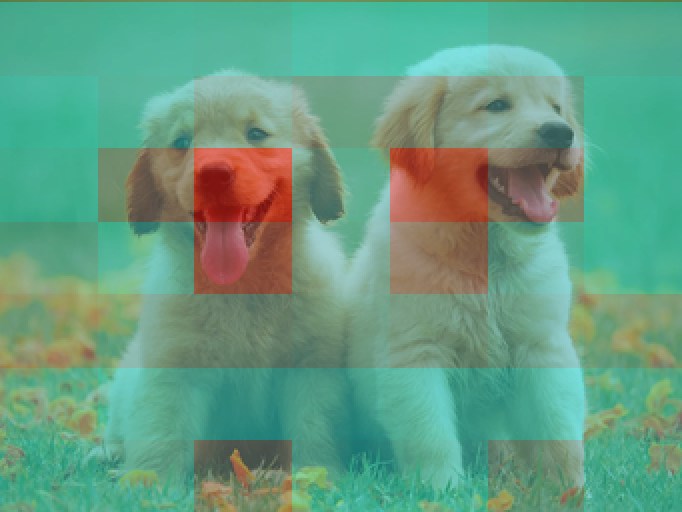
Attention visualization for images
Just like the original Vision Transformer (see the model "Vision Transformer Trained on ImageNet Competition Data"), the image feature extractor divides the input images in 7x7 patches and performs self-attention on a set of 50 vectors: 49 vectors, or "tokens," representing the 7x7 patches and an additional one, a "feature extraction token," that is eventually used to produce the final feature representation of the image. Thus the attention procedure for this model can be visualized by inspecting the attention weights between the feature extraction token and the patch tokens. Define a test image:
Extract the attention weights used for the last block of self-attention:
Extract the attention weights between the feature extraction token and the input patches. These weights can be interpreted as which patches in the original image the net is "looking at" in order to perform the feature extraction:
Reshape the weights as a 3D array of 12 7x7 matrices. Each matrix corresponds to an attention head, while each element of the matrices corresponds to a patch in the original image:
Visualize the attention weight matrices. Patches with higher values (red) are what is mostly being "looked at" for each attention head:
Define a function to visualize the attention matrix on an image:
Visualize the mean attention across all the attention heads:
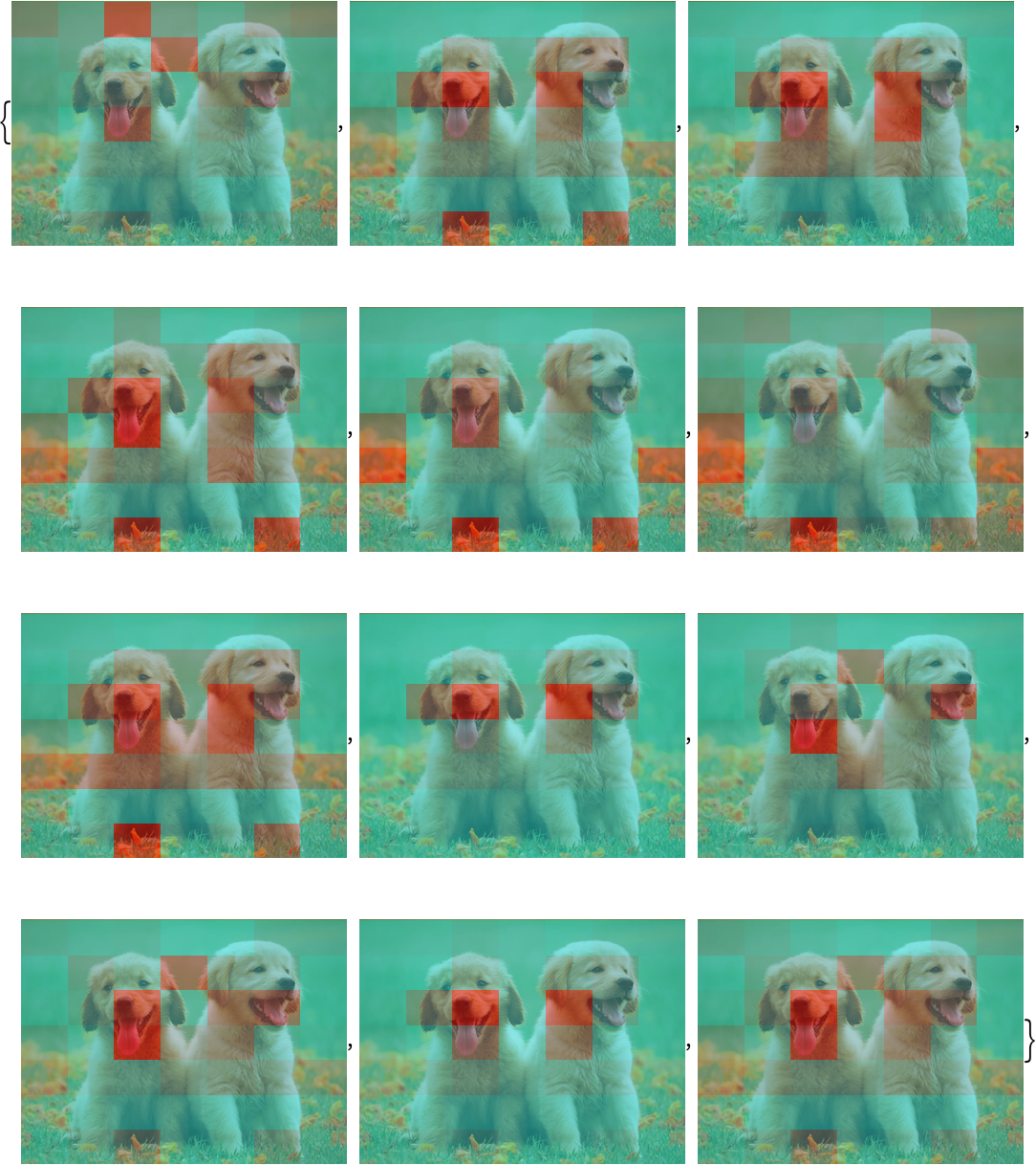
Visualize each attention head separately:
Attention visualization for text
The text feature extractor tokenizes the input string prepending and appending the special tokens StartOfString and EndOfString and then performs causal self-attention on the token embedding vectors. After the self-attention stack, the last vector (corresponding to the token EndOfString) is used to obtain the final feature representation of the text. Thus the attention procedure for this model can be visualized by inspecting the attention weights between the last vector and the previous ones. Define a test string:
Extract the NetEncoder of the net to encode the string:
Extract the list of available tokens and inspect how the input string was tokenized. Even though the BPE tokenization generally segments the input into subwords, it's common to observe that all tokens correspond to full words. Also observe that the StartOfString and EndOfString tokens are added automatically:
Feed the string to the net and extract the attention weights used for the last block of self-attention:
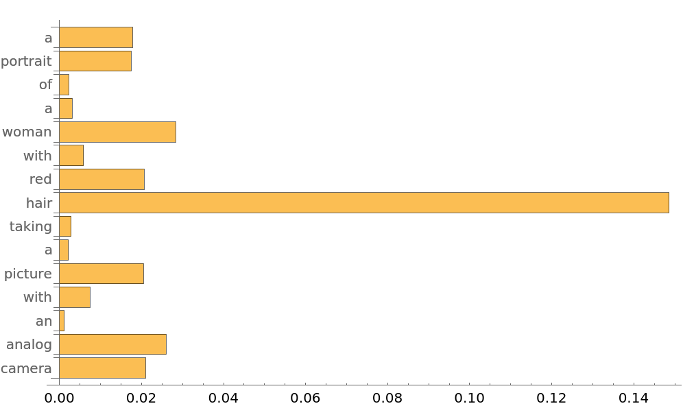
Extract the attention weights between the last vector and the previous ones, leaving the initial vector corresponding to StartOfString out. These weights can be interpreted as which tokens in the original sentence the net is "looking at" in order to perform the feature extraction:
Inspect the average attention weights for each token across the attention heads. Observe that the token the net is mostly focused on is "hair":
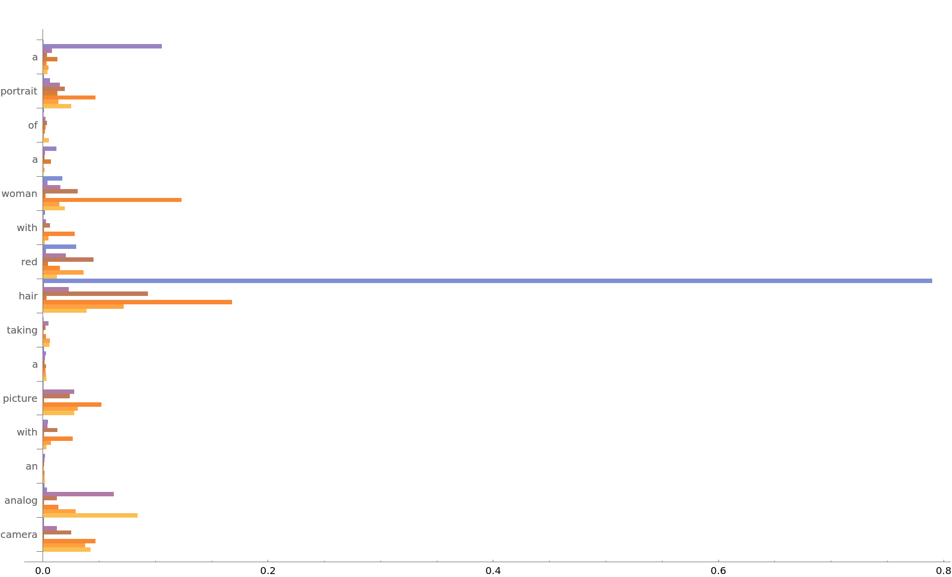
Visualize each head separately:
Extract the attention weights for all 12 attention layers:
Compute the average across all heads, leaving the StartOfString token out:
Define a function to visualize the attention weights:
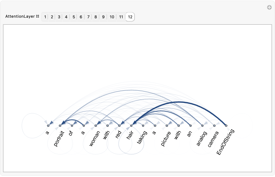
Explore the attention weights for every layer. A thicker arrow pointing from token A to token B indicates that the layer is paying attention to token B when generating the vector corresponding to token A:
Transfer learning
Use the pre-trained model to build a classifier for telling apart indoor and outdoor photos. Create a test set and a training set:
Remove the last linear layer from the pre-trained net:
Create a new net composed of the pre-trained net followed by a linear layer and a softmax layer:
Train on the dataset, freezing all the weights except for those in the "linearNew" layer (use TargetDevice -> "GPU" for training on a GPU):
Perfect accuracy is obtained on the test set:
Net information
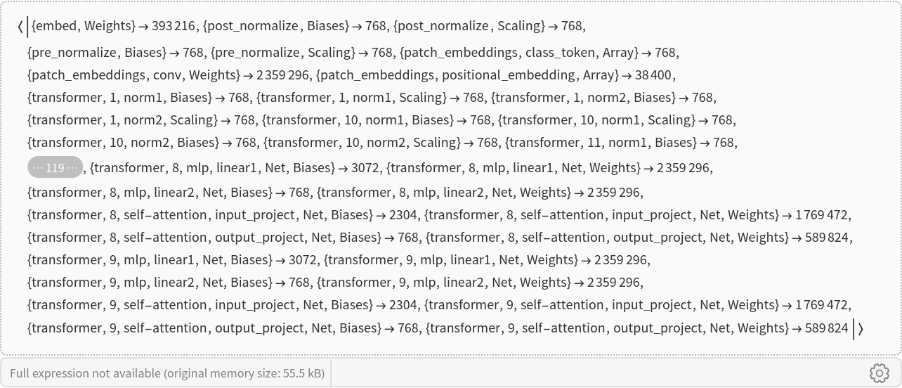
Inspect the number of parameters of all arrays in the net:
Obtain the total number of parameters:
Obtain the layer type counts:

![NetModel["OpenCLIP Multi-domain Feature Extractor Trained on LAION-2B Data", "ParametersInformation"]](https://www.wolframcloud.com/obj/resourcesystem/images/6a8/6a872ecb-2ca9-4925-b863-fba48d127123/0d5dd31cec506ab2.png)
![NetModel[{"OpenCLIP Multi-domain Feature Extractor Trained on LAION-2B Data", "InputDomain" -> "Text", "Architecture" -> "ViT-B/16"}]](https://www.wolframcloud.com/obj/resourcesystem/images/6a8/6a872ecb-2ca9-4925-b863-fba48d127123/4d59c477f38fd575.png)

![NetModel[{"OpenCLIP Multi-domain Feature Extractor Trained on LAION-2B Data", "InputDomain" -> "Text", "Architecture" -> "ViT-B/16"}, "UninitializedEvaluationNet"]](https://www.wolframcloud.com/obj/resourcesystem/images/6a8/6a872ecb-2ca9-4925-b863-fba48d127123/3ce0ae94735f5a0c.png)
![textEmbedding = NetModel[{"OpenCLIP Multi-domain Feature Extractor Trained on LAION-2B Data", "InputDomain" -> "Text"}]["Challenge accepted!"];](https://www.wolframcloud.com/obj/resourcesystem/images/6a8/6a872ecb-2ca9-4925-b863-fba48d127123/4ca632c2ca0d1cf3.png)
![(* Evaluate this cell to get the example input *) CloudGet["https://www.wolframcloud.com/obj/f96193b5-d0d1-4daa-9e6a-d94b25133718"]](https://www.wolframcloud.com/obj/resourcesystem/images/6a8/6a872ecb-2ca9-4925-b863-fba48d127123/6a47020272d57c99.png)
![(* Evaluate this cell to get the example input *) CloudGet["https://www.wolframcloud.com/obj/c73d854f-5ce6-4b76-a3c4-46c6bcd941d1"]](https://www.wolframcloud.com/obj/resourcesystem/images/6a8/6a872ecb-2ca9-4925-b863-fba48d127123/4445ab4061fd369a.png)
![FeatureSpacePlot[
Thread[NetModel[{"OpenCLIP Multi-domain Feature Extractor Trained on LAION-2B Data", "InputDomain" -> "Image"}][imgs, NetPort[{"embed", "Output"}]] -> imgs],
LabelingSize -> 70,
LabelingFunction -> Callout,
ImageSize -> 600,
AspectRatio -> 0.9,
RandomSeeding -> 123456
]](https://www.wolframcloud.com/obj/resourcesystem/images/6a8/6a872ecb-2ca9-4925-b863-fba48d127123/6befbf7629cc1480.png)
![FeatureSpacePlot[
Thread[NetModel[{"OpenCLIP Multi-domain Feature Extractor Trained on LAION-2B Data", "InputDomain" -> "Text"}][sentences, NetPort[{"embed", "Output"}]] -> sentences]
, LabelingFunction -> Callout, LabelingSize -> {120, 70}, ImageSize -> 600, PlotMarkers -> {Automatic, Scaled[0.01]}, RandomSeeding -> 123465]](https://www.wolframcloud.com/obj/resourcesystem/images/6a8/6a872ecb-2ca9-4925-b863-fba48d127123/6e32e40fdfefa446.png)
![(* Evaluate this cell to get the example input *) CloudGet["https://www.wolframcloud.com/obj/a8cc9424-a808-494c-9878-45322e441c91"]](https://www.wolframcloud.com/obj/resourcesystem/images/6a8/6a872ecb-2ca9-4925-b863-fba48d127123/4349102164de893c.png)
![textFeatures = NetModel[{"OpenCLIP Multi-domain Feature Extractor Trained on LAION-2B Data", "InputDomain" -> "Text", "Architecture" -> "ViT-B/16"}][descriptions];
imgFeatures = NetModel[{"OpenCLIP Multi-domain Feature Extractor Trained on LAION-2B Data", "InputDomain" -> "Image", "Architecture" -> "ViT-B/16"}][img];](https://www.wolframcloud.com/obj/resourcesystem/images/6a8/6a872ecb-2ca9-4925-b863-fba48d127123/68c9a61666aac2ef.png)
![Dataset@SortBy[
Thread[{descriptions, First@DistanceMatrix[{imgFeatures}, textFeatures, DistanceFunction -> CosineDistance]}], Last]](https://www.wolframcloud.com/obj/resourcesystem/images/6a8/6a872ecb-2ca9-4925-b863-fba48d127123/031af53b995157e8.png)

![textEmbeddings = NetModel[
"OpenCLIP Multi-domain Feature Extractor Trained on LAION-2B Data", "InputDomain" -> "Text"][labelTemplates];](https://www.wolframcloud.com/obj/resourcesystem/images/6a8/6a872ecb-2ca9-4925-b863-fba48d127123/6793cc16bc12b952.png)
![imgFeatures = NetModel[
"OpenCLIP Multi-domain Feature Extractor Trained on LAION-2B Data", "InputDomain" -> "Image"][img];](https://www.wolframcloud.com/obj/resourcesystem/images/6a8/6a872ecb-2ca9-4925-b863-fba48d127123/36b41aab00cfb1fb.png)
![SortBy[Rule @@@ MapAt[labelTemplates[[#]] &, Nearest[textEmbeddings -> {"Index", "Distance"}, imgFeatures, 10, DistanceFunction -> CosineDistance], {All, 1}], Last]](https://www.wolframcloud.com/obj/resourcesystem/images/6a8/6a872ecb-2ca9-4925-b863-fba48d127123/2a73c23a9bd1d7a9.png)

![imageEmbeddings = NetModel[
"OpenCLIP Multi-domain Feature Extractor Trained on LAION-2B Data", "InputDomain" -> "Image"][testData[[All, 1]], TargetDevice -> "CPU"];](https://www.wolframcloud.com/obj/resourcesystem/images/6a8/6a872ecb-2ca9-4925-b863-fba48d127123/0f30cf599c08c6a9.png)
![(* Evaluate this cell to get the example input *) CloudGet["https://www.wolframcloud.com/obj/80b0126c-3262-4c5e-8195-fc94034a0021"]](https://www.wolframcloud.com/obj/resourcesystem/images/6a8/6a872ecb-2ca9-4925-b863-fba48d127123/2f77551b3d077894.png)
![attentionMatrix = Transpose@
NetModel[{"OpenCLIP Multi-domain Feature Extractor Trained on LAION-2B Data", "InputDomain" -> "Image"}][testImage, NetPort[{"transformer", -1, "self-attention", "attention", "AttentionWeights"}]];](https://www.wolframcloud.com/obj/resourcesystem/images/6a8/6a872ecb-2ca9-4925-b863-fba48d127123/701ef555663fa865.png)
![visualizeAttention[img_Image, attentionMatrix_] := Block[{heatmap, wh},
wh = ImageDimensions[img];
heatmap = ImageApply[{#, 1 - #, 1 - #} &, ImageAdjust@Image[attentionMatrix]];
heatmap = ImageResize[heatmap, wh*256/Min[wh]];
ImageCrop[ImageCompose[img, {ColorConvert[heatmap, "RGB"], 0.4}], ImageDimensions[heatmap]]
]](https://www.wolframcloud.com/obj/resourcesystem/images/6a8/6a872ecb-2ca9-4925-b863-fba48d127123/6b0ca1d495426e4b.png)
![netEnc = NetExtract[
NetModel[{"OpenCLIP Multi-domain Feature Extractor Trained on LAION-2B Data", "InputDomain" -> "Text"}], "Input"]](https://www.wolframcloud.com/obj/resourcesystem/images/6a8/6a872ecb-2ca9-4925-b863-fba48d127123/324920f981277cd3.png)
![attentionMatrix = Transpose@
NetModel[{"OpenCLIP Multi-domain Feature Extractor Trained on LAION-2B Data", "InputDomain" -> "Text"}][text, NetPort[{"transformer", -1, "self-attention", "attention", "AttentionWeights"}]];
Dimensions[attentionMatrix]](https://www.wolframcloud.com/obj/resourcesystem/images/6a8/6a872ecb-2ca9-4925-b863-fba48d127123/4c447f0926f005ff.png)
![allAttentionWeights = Transpose[
Values@NetModel[{"OpenCLIP Multi-domain Feature Extractor Trained on LAION-2B Data", "InputDomain" -> "Text"}][text, spec], 2 <-> 3];
Dimensions[allAttentionWeights]](https://www.wolframcloud.com/obj/resourcesystem/images/6a8/6a872ecb-2ca9-4925-b863-fba48d127123/2d6536353959c8c9.png)
![visualizeTokenAttention[attnMatrix_] := Block[{g, style},
g = WeightedAdjacencyGraph[attnMatrix];
style = Thread@Directive[
Arrowheads[.02],
Thickness /@ (Rescale[AnnotationValue[g, EdgeWeight]]/200),
Opacity /@ Rescale@AnnotationValue[g, EdgeWeight]
];
Graph[g, GraphLayout -> "LinearEmbedding", EdgeStyle -> Thread[EdgeList[g] -> style], VertexLabels -> Thread[Range[Length@Rest[tokens]] -> Map[Rotate[Style[Text[#], 12, Bold], 60 Degree] &, Rest[tokens]]], VertexCoordinates -> Table[{i, 0}, {i, Length[attnMatrix]}], ImageSize -> Large]
]](https://www.wolframcloud.com/obj/resourcesystem/images/6a8/6a872ecb-2ca9-4925-b863-fba48d127123/03aee0a7efc2e282.png)
![Manipulate[
visualizeTokenAttention@
avgAttentionWeights[[i]], {{i, 12, "AttentionLayer #"}, Range[12]}, ControlType -> SetterBar]](https://www.wolframcloud.com/obj/resourcesystem/images/6a8/6a872ecb-2ca9-4925-b863-fba48d127123/2dd1791256770ff3.png)
![(* Evaluate this cell to get the example input *) CloudGet["https://www.wolframcloud.com/obj/31006b39-cd75-4060-85d9-4278468b2f50"]](https://www.wolframcloud.com/obj/resourcesystem/images/6a8/6a872ecb-2ca9-4925-b863-fba48d127123/1e00c98d17eb827a.png)
![(* Evaluate this cell to get the example input *) CloudGet["https://www.wolframcloud.com/obj/e6ddd9f4-dcff-4c19-970f-28bc1b779aa7"]](https://www.wolframcloud.com/obj/resourcesystem/images/6a8/6a872ecb-2ca9-4925-b863-fba48d127123/5221374ff954a12b.png)
![tempNet = NetModel[{"OpenCLIP Multi-domain Feature Extractor Trained on LAION-2B Data", "InputDomain" -> "Image"}]](https://www.wolframcloud.com/obj/resourcesystem/images/6a8/6a872ecb-2ca9-4925-b863-fba48d127123/6512a9288bb57c92.png)
![Information[
NetModel[
"OpenCLIP Multi-domain Feature Extractor Trained on LAION-2B Data"], "ArraysElementCounts"]](https://www.wolframcloud.com/obj/resourcesystem/images/6a8/6a872ecb-2ca9-4925-b863-fba48d127123/32515d55427a340c.png)
![Information[
NetModel[
"OpenCLIP Multi-domain Feature Extractor Trained on LAION-2B Data"], "ArraysTotalElementCount"]](https://www.wolframcloud.com/obj/resourcesystem/images/6a8/6a872ecb-2ca9-4925-b863-fba48d127123/0c7fdf07734b8b27.png)
![Information[
NetModel[
"OpenCLIP Multi-domain Feature Extractor Trained on LAION-2B Data"], "LayerTypeCounts"]](https://www.wolframcloud.com/obj/resourcesystem/images/6a8/6a872ecb-2ca9-4925-b863-fba48d127123/0273eb65e10f10bd.png)
