Multi-scale Context Aggregation Net
Trained on
Cityscapes Data
Released in 2016, this is the first model featuring a systematic use of dilated convolutions for pixel-wise classification. A context aggregation module featuring convolutions with exponentially increasing dilations is appended to a VGG-style front end.
Number of layers: 58 |
Parameter count: 134,460,595 |
Trained size: 538 MB |
Examples
Resource retrieval
Get the pre-trained net:
Evaluation function
Write an evaluation function to handle padding and tiling of the input image:
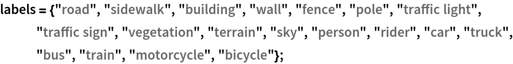
Label list
Define the label list for this model. Integers in the model’s output correspond to elements in the label list:
Basic usage
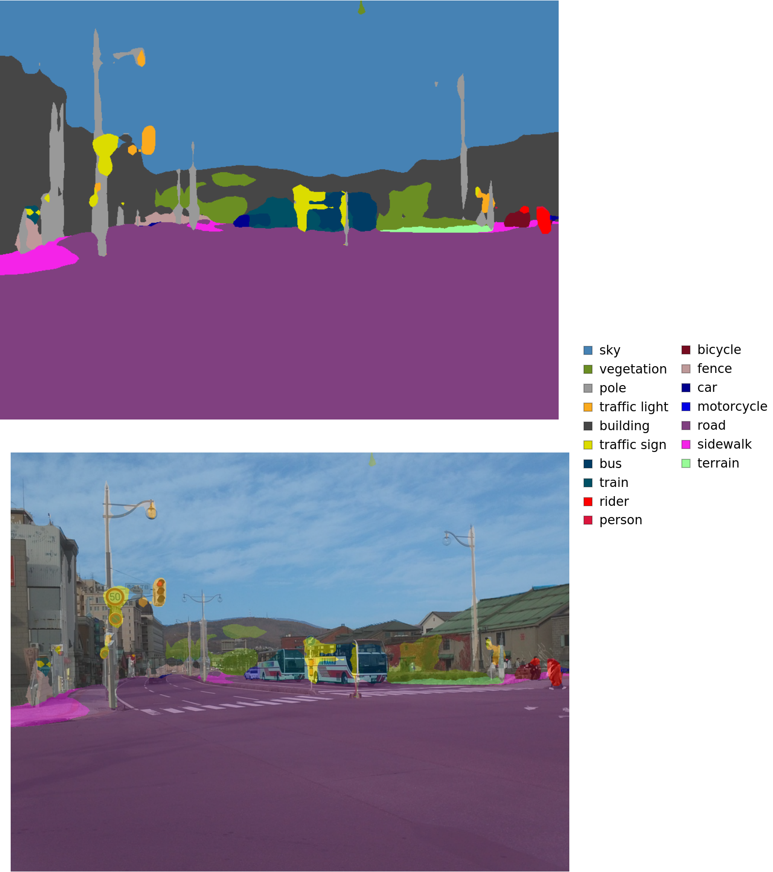
Obtain a segmentation mask for a given image:
Inspect which classes are detected:
Visualize the mask:
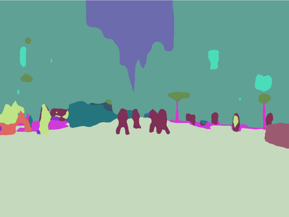
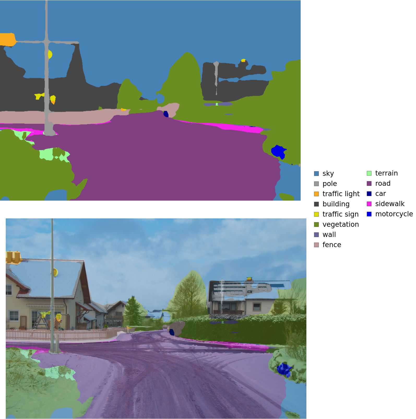
Advanced visualization
Associate classes to colors using the standard Cityscapes palette:
Write a function to overlap the image and the mask with a legend:
Inspect the results:
Net information
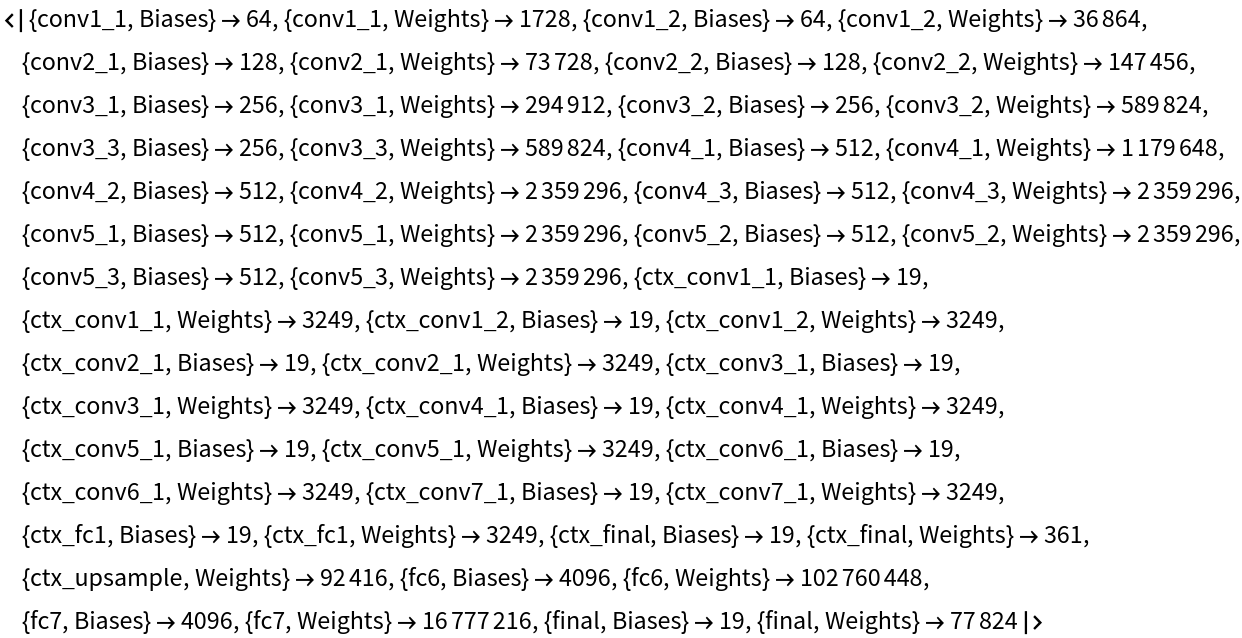
Inspect the number of parameters of all arrays in the net:
Obtain the total number of parameters:
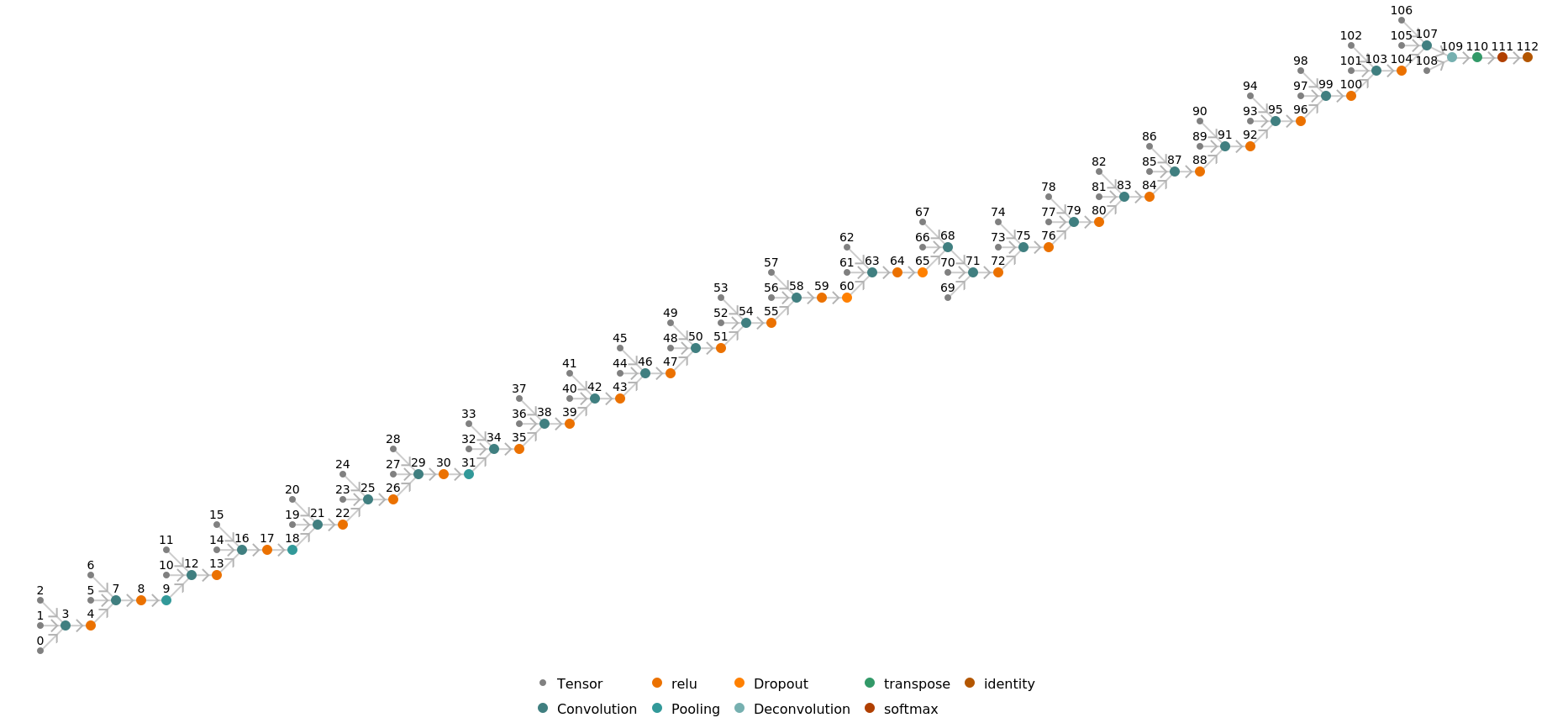
Obtain the layer type counts:
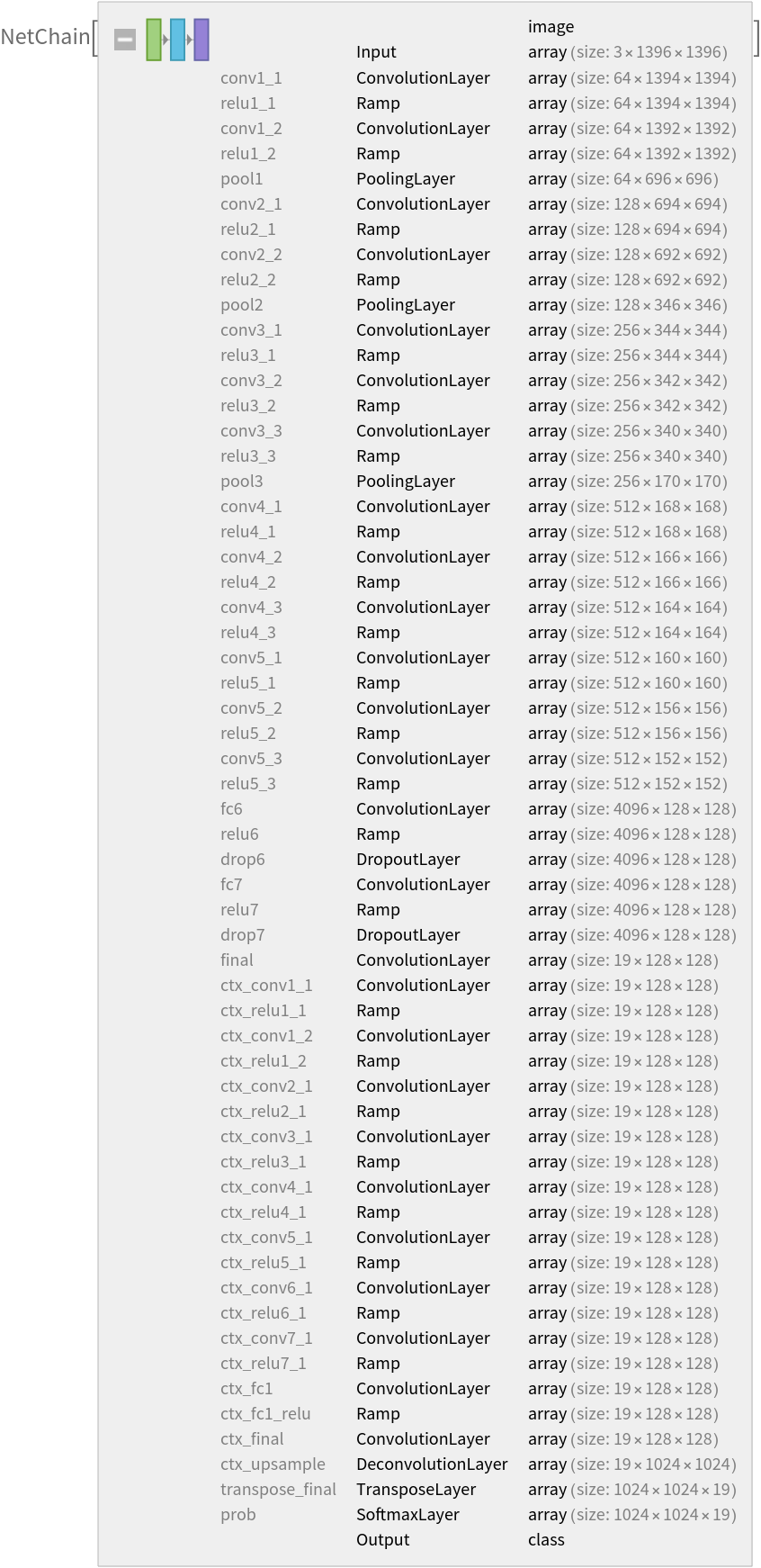
Display the summary graphic:
Export to MXNet
Export the net into a format that can be opened in MXNet:
Export also creates a net.params file containing parameters:
Get the size of the parameter file:
The size is similar to the byte count of the resource object:
Represent the MXNet net as a graph:
Requirements
Wolfram Language
11.3
(March 2018)
or above
Resource History
Reference
![netevaluate[img_, device_ : "CPU"] := Block[
{net, marginImg, inputSize, windowSize, imgPad, imgSize, takeSpecs, tiles, marginTile, prob},
(* Parameters *) net = NetModel[
"Multi-scale Context Aggregation Net Trained on Cityscapes \
Data"];
marginImg = 186;
inputSize = 1396;
windowSize = inputSize - 2*marginImg;
(* Pad and tile input *) imgPad = ImagePad[img, marginImg, "Reflected"];
imgSize = ImageDimensions[imgPad];
takeSpecs = Table[
{{i, i + inputSize - 1}, {j, j + inputSize - 1}},
{i, 1, imgSize[[2]] - 2*marginImg, windowSize},
{j, 1, imgSize[[1]] - 2*marginImg, windowSize}
];
tiles = Map[ImageTake[imgPad, Sequence @@ #] &, takeSpecs, {2}];
(* Make all tiles 1396x1396 *) marginTile = windowSize - Mod[imgSize - 2*marginImg, windowSize];
tiles = MapAt[ImagePad[#, {{0, marginTile[[1]]}, {0, 0}}, "Reflected"] &, tiles, {All, -1}];
tiles = MapAt[ImagePad[#, {{0, 0}, {marginTile[[2]], 0}}, "Reflected"] &, tiles, {-1, All}];
(* Run net on tiles *) prob = net[Flatten@tiles, None, TargetDevice -> device];
prob = ArrayFlatten@
ArrayReshape[prob, Join[Dimensions@tiles, {1024, 1024, 19}]];
(* Trim additional tile margin *) prob = Take[prob, Sequence @@ Reverse[ImageDimensions@img], All];
(* Predict classes *)
NetExtract[net, "Output"]@prob
]](https://www.wolframcloud.com/obj/resourcesystem/images/507/507d3556-b3e6-423a-aec0-e245f6087ff7/17ede5ec96969b8e.png)
![(* Evaluate this cell to get the example input *) CloudGet["https://www.wolframcloud.com/obj/af44f3b3-06e6-4a26-a6fb-a3e9c55ba5bf"]](https://www.wolframcloud.com/obj/resourcesystem/images/507/507d3556-b3e6-423a-aec0-e245f6087ff7/4511df487986de0d.png)
![colors = Apply[
RGBColor, {{128, 64, 128}, {244, 35, 232}, {70, 70, 70}, {102, 102, 156}, {190, 153, 153}, {153, 153, 153}, {250, 170, 30}, {220, 220, 0}, {107, 142, 35}, {152, 251, 152}, {70, 130, 180}, {220, 20, 60}, {255, 0, 0}, {0, 0, 142}, {0, 0, 70}, {0, 60, 100}, {0, 80, 100}, {0, 0, 230}, {119, 11, 32}}/255., {1}]](https://www.wolframcloud.com/obj/resourcesystem/images/507/507d3556-b3e6-423a-aec0-e245f6087ff7/4bffdc176a0b6abe.png)
![result[img_, device_ : "CPU"] := Block[
{mask, classes, maskPlot, composition},
mask = netevaluate[img, device];
classes = DeleteDuplicates[Flatten@mask];
maskPlot = Colorize[mask, ColorRules -> indexToColor];
composition = ImageCompose[img, {maskPlot, 0.5}];
Legended[
Row[Image[#, ImageSize -> Large] & /@ {maskPlot, composition}], SwatchLegend[indexToColor[[classes, 2]], labels[[classes]]]]
]](https://www.wolframcloud.com/obj/resourcesystem/images/507/507d3556-b3e6-423a-aec0-e245f6087ff7/2fd8c73d79528c04.png)
![(* Evaluate this cell to get the example input *) CloudGet["https://www.wolframcloud.com/obj/8bc73a3e-85f3-41b9-ba3f-5bcc30d5c51a"]](https://www.wolframcloud.com/obj/resourcesystem/images/507/507d3556-b3e6-423a-aec0-e245f6087ff7/541a44d421ac8f99.png)
![(* Evaluate this cell to get the example input *) CloudGet["https://www.wolframcloud.com/obj/2ccc2de2-f781-4451-9519-d230aa76f764"]](https://www.wolframcloud.com/obj/resourcesystem/images/507/507d3556-b3e6-423a-aec0-e245f6087ff7/717f553928ff1c79.png)
![(* Evaluate this cell to get the example input *) CloudGet["https://www.wolframcloud.com/obj/62d0a32e-c5f7-4499-a7d1-1e6a3de95bb6"]](https://www.wolframcloud.com/obj/resourcesystem/images/507/507d3556-b3e6-423a-aec0-e245f6087ff7/5523a2766fdf852f.png)