Dilated ResNet-22
Trained on
Cityscapes Data
Released in 2017, this architecure combines the technique of dilated convolutions with the paradigm of residual networks, outperforming their nonrelated counterparts in image classification and semantic segmentation.
Number of layers: 86 |
Parameter count: 15,994,691 |
Trained size: 64 MB |
Examples
Resource retrieval
Get the pre-trained net:
Evaluation function
Write an evaluation function to handle net reshaping and resampling of input and output:
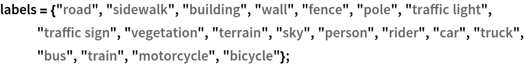
Label list
Define the label list for this model. Integers in the model’s output correspond to elements in the label list:
Basic usage
Obtain a segmentation mask for a given image:
Inspect which classes are detected:
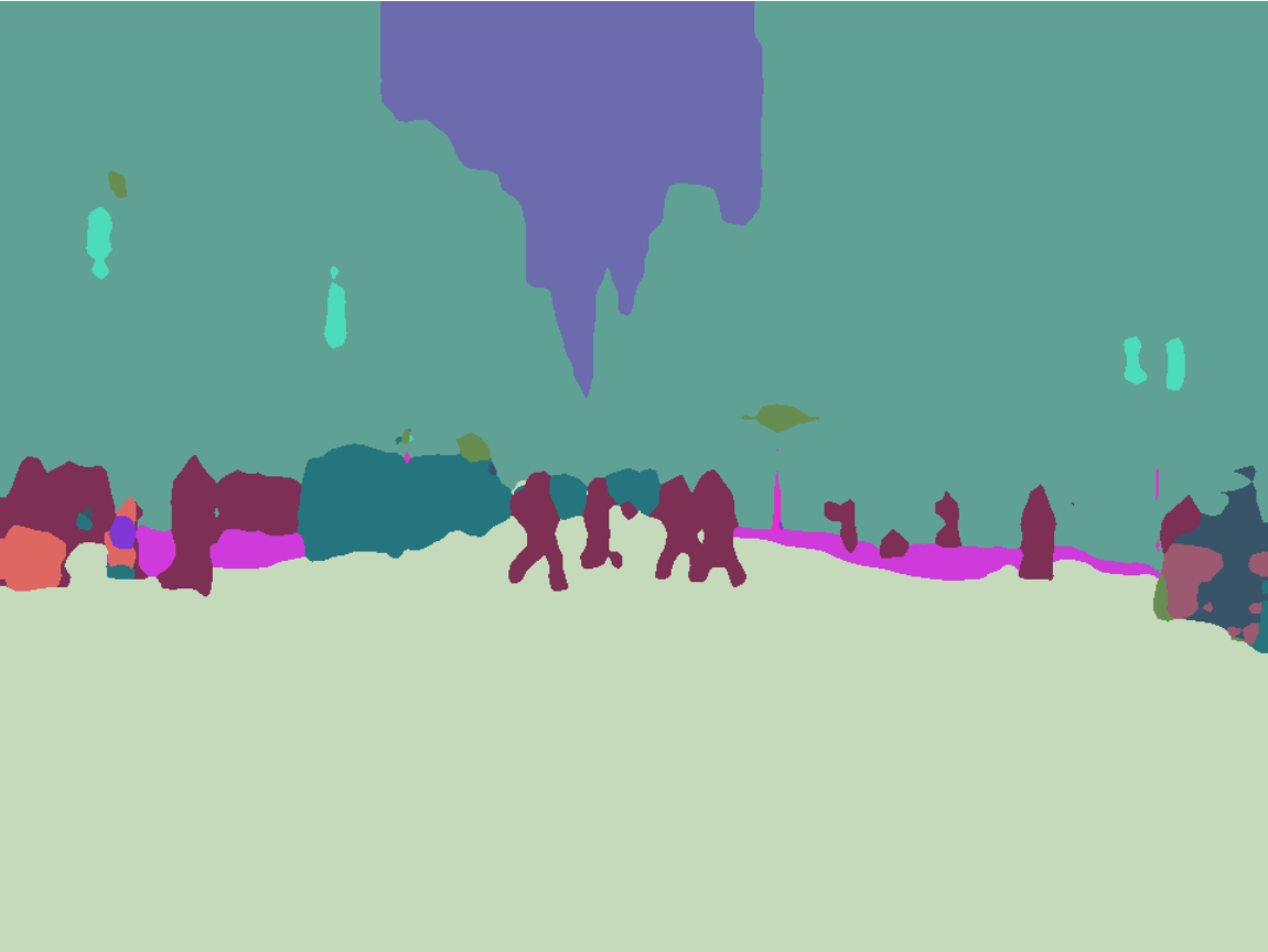
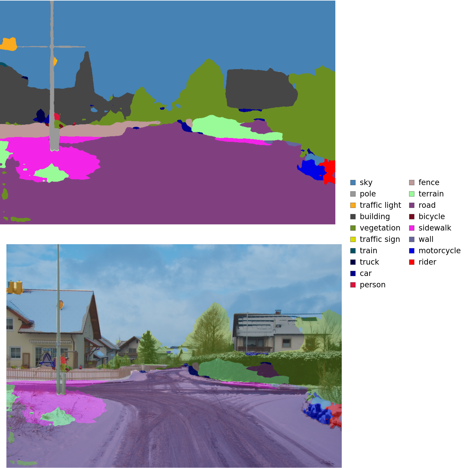
Visualize the mask:
Advanced visualization
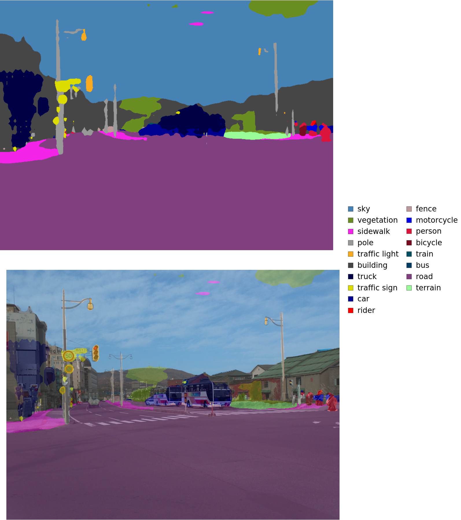
Associate classes to colors using the standard Cityscapes palette:
Write a function to overlap the image and the mask with a legend:
Inspect the results:
Net information
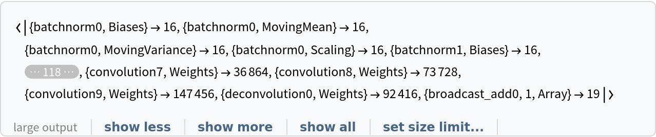
Inspect the number of parameters of all arrays in the net:
Obtain the total number of parameters:
Obtain the layer type counts:
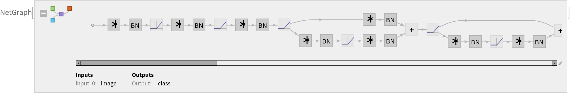
Display the summary graphic:
Export to MXNet
Export the net into a format that can be opened in MXNet:
Export also creates a net.params file containing parameters:
Get the size of the parameter file:
The size is similar to the byte count of the resource object:
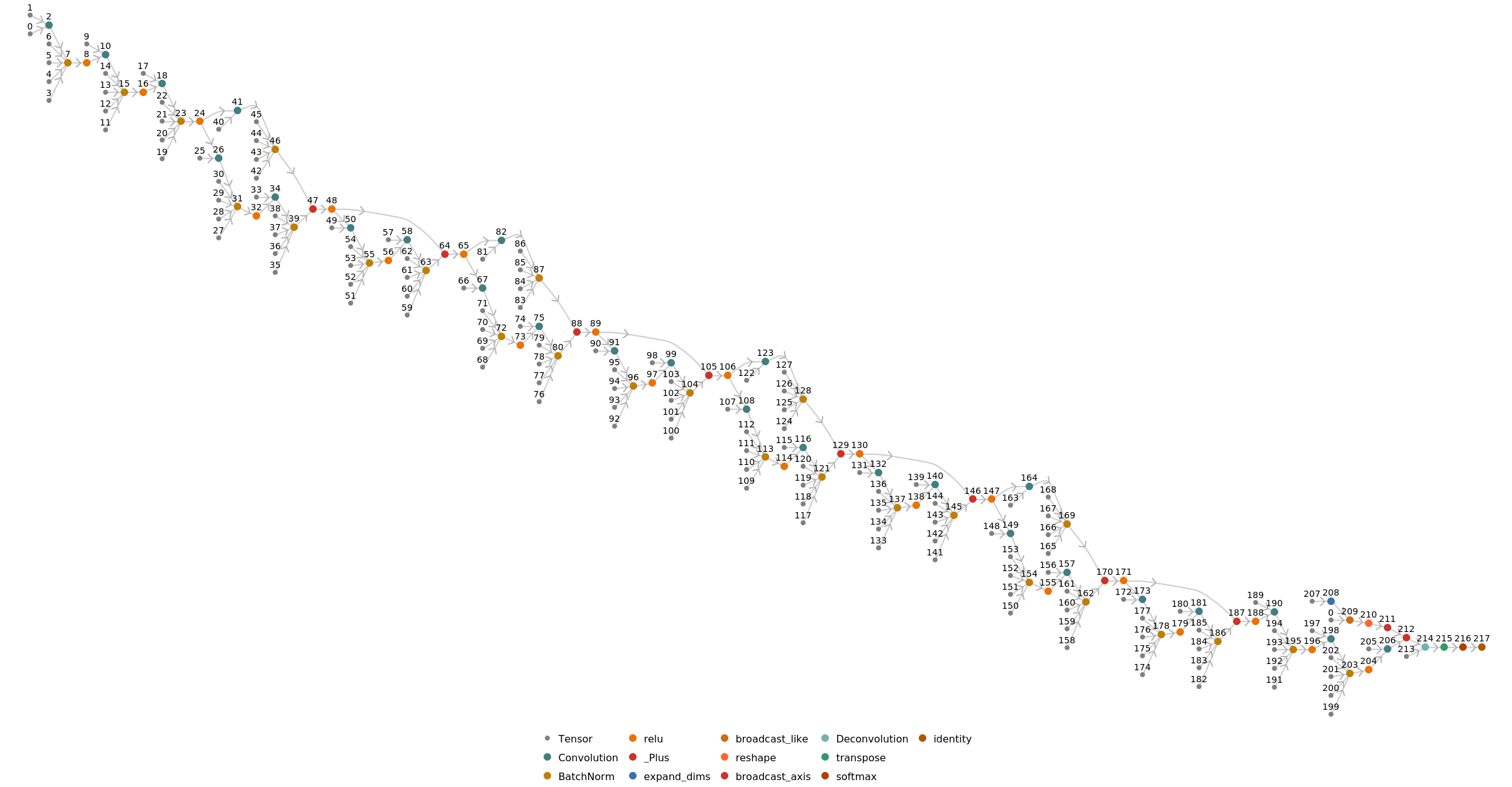
Represent the MXNet net as a graph:
Requirements
Wolfram Language
11.3
(March 2018)
or above
Resource History
Reference
![netevaluate[img_, device_ : "CPU"] := Block[
{net, encData, dec, mean, var, prob},
net = NetModel["Dilated ResNet-22 Trained on Cityscapes Data"];
encData = Normal@NetExtract[net, "input_0"];
dec = NetExtract[net, "Output"];
{mean, var} = Lookup[encData, {"MeanImage", "VarianceImage"}];
NetReplacePart[net,
{"input_0" -> NetEncoder[{"Image", ImageDimensions@img, "MeanImage" -> mean, "VarianceImage" -> var}], "Output" -> dec}
][img, TargetDevice -> device]
]](https://www.wolframcloud.com/obj/resourcesystem/images/3e8/3e883192-f67d-4da9-923a-f9fddc4dc7ab/1e019412ebba0847.png)
![(* Evaluate this cell to get the example input *) CloudGet["https://www.wolframcloud.com/obj/90161845-03f3-4235-adfc-5b9de58bec2b"]](https://www.wolframcloud.com/obj/resourcesystem/images/3e8/3e883192-f67d-4da9-923a-f9fddc4dc7ab/7dfcf213899fba36.png)
![colors = Apply[
RGBColor, {{128, 64, 128}, {244, 35, 232}, {70, 70, 70}, {102, 102, 156}, {190, 153, 153}, {153, 153, 153}, {250, 170, 30}, {220, 220, 0}, {107, 142, 35}, {152, 251, 152}, {70, 130, 180}, {220, 20, 60}, {255, 0, 0}, {0, 0, 142}, {0, 0, 70}, {0, 60, 100}, {0, 80, 100}, {0, 0, 230}, {119, 11, 32}}/255., {1}]](https://www.wolframcloud.com/obj/resourcesystem/images/3e8/3e883192-f67d-4da9-923a-f9fddc4dc7ab/42aff53bcae8af9f.png)
![result[img_, device_ : "CPU"] := Block[
{mask, classes, maskPlot, composition},
mask = netevaluate[img, device];
classes = DeleteDuplicates[Flatten@mask];
maskPlot = Colorize[mask, ColorRules -> indexToColor];
composition = ImageCompose[img, {maskPlot, 0.5}];
Legended[
Row[Image[#, ImageSize -> Large] & /@ {maskPlot, composition}], SwatchLegend[indexToColor[[classes, 2]], labels[[classes]]]]
]](https://www.wolframcloud.com/obj/resourcesystem/images/3e8/3e883192-f67d-4da9-923a-f9fddc4dc7ab/21ed88b928125bc7.png)
![(* Evaluate this cell to get the example input *) CloudGet["https://www.wolframcloud.com/obj/9e30aff4-8c11-459e-81c7-4d34b6f982f5"]](https://www.wolframcloud.com/obj/resourcesystem/images/3e8/3e883192-f67d-4da9-923a-f9fddc4dc7ab/3aa892612115ad9e.png)
![(* Evaluate this cell to get the example input *) CloudGet["https://www.wolframcloud.com/obj/d080db18-e42f-47ec-b9d4-8e14a2d67314"]](https://www.wolframcloud.com/obj/resourcesystem/images/3e8/3e883192-f67d-4da9-923a-f9fddc4dc7ab/5d4719d64fc32b86.png)
![(* Evaluate this cell to get the example input *) CloudGet["https://www.wolframcloud.com/obj/3bfec9cc-4f18-438a-8040-41fb5ad2c207"]](https://www.wolframcloud.com/obj/resourcesystem/images/3e8/3e883192-f67d-4da9-923a-f9fddc4dc7ab/732d3d83ad041c3d.png)