SSD-MobileNet V2
Trained on
MS-COCO Data
Released in 2019, this model is a single-stage object detection model that goes straight from image pixels to bounding box coordinates and class probabilities. The model architecture is based on inverted residual structure where the input and output of the residual block are thin bottleneck layers as opposed to traditional residual models. Moreover, nonlinearities are removed from intermediate layers and lightweight depthwise convolution is used. This model is part of the Tensorflow object detection API.
Number of layers: 267 |
Parameter count: 15,291,106 |
Trained size: 63 MB |
Examples
Resource retrieval
Get the pre-trained net:
Evaluation function
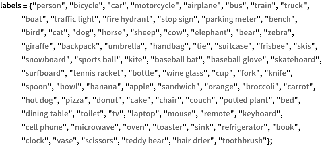
Define the label list for this model. Integers in the model's output correspond to elements in the label list:
Write an evaluation function to scale the result to the input image size and suppress the least probable detections:
Basic usage
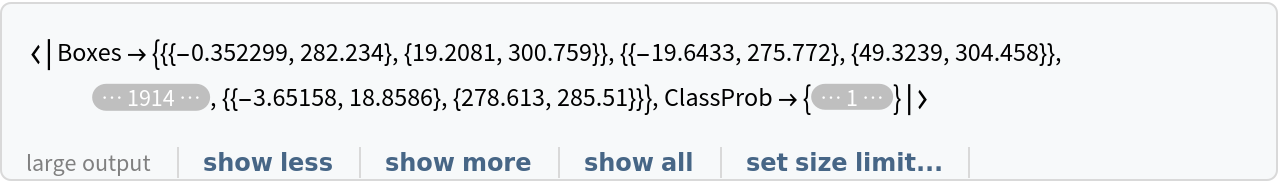
Obtain the detected bounding boxes with their corresponding classes and confidences for a given image:
Inspect which classes are detected:
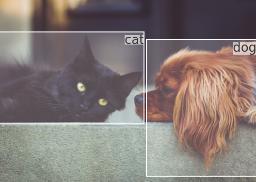
Visualize the detection:
Network result
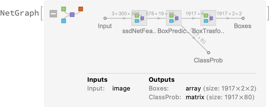
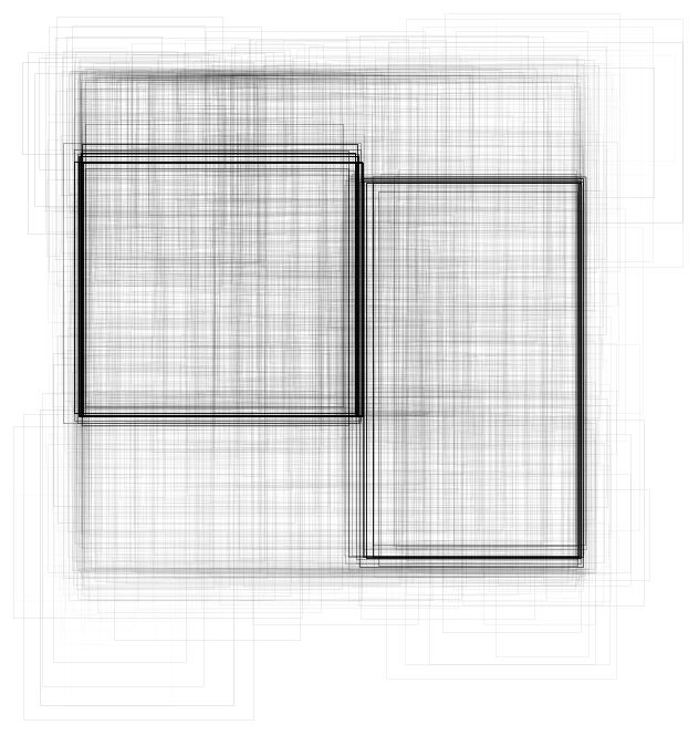
The network computes 1,917 bounding boxes and the probability that the objects in each box are of any given class:
Visualize all the boxes predicted by the net scaled by their “objectness” measures:
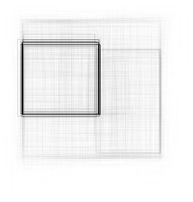
Visualize all the boxes scaled by the probability that they contain a cat:
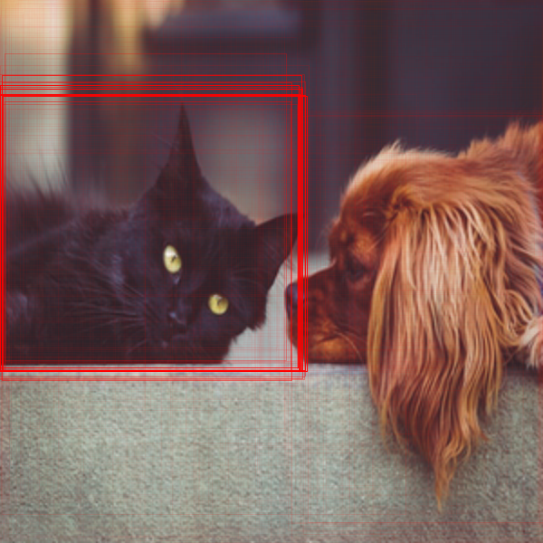
Superimpose the cat prediction on top of the scaled input received by the net:
Advanced visualization
Write a function to apply a custom styling to the result of the detection:
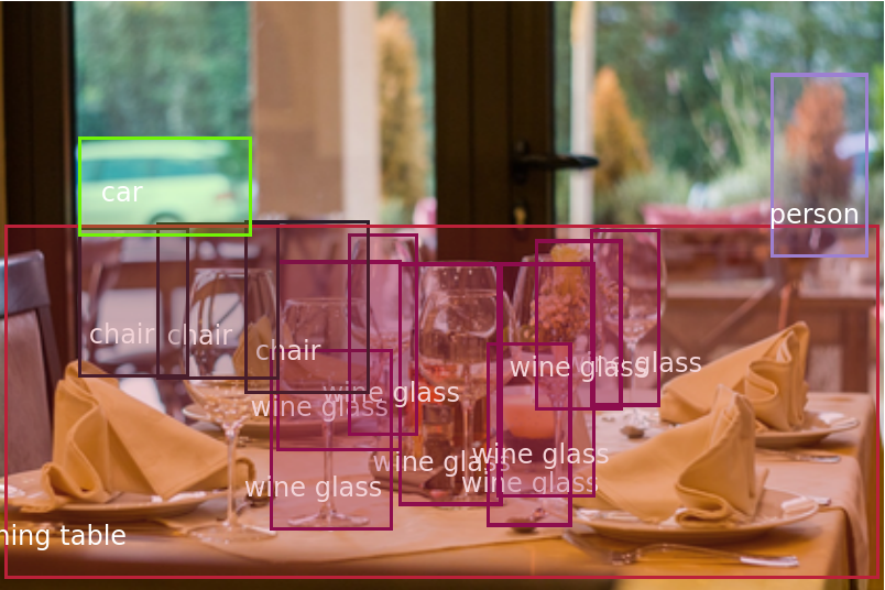
Visualize multiple objects, using a different color for each class:
Net information
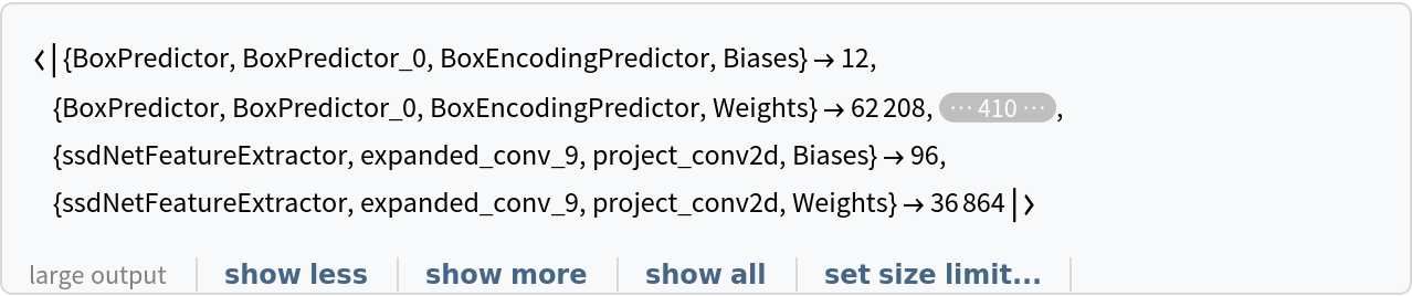
Inspect the number of parameters of all arrays in the net:
Obtain the total number of parameters:
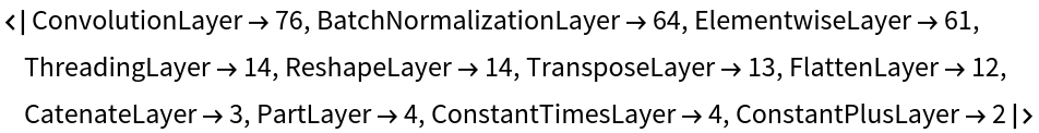
Obtain the layer type counts:
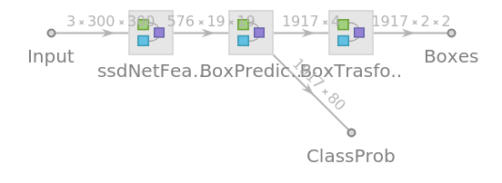
Display the summary graphic:
Export to MXNet
Export the net into a format that can be opened in MXNet:
Export also creates a net.params file containing parameters:
Get the size of the parameter file:
The size is similar to the byte count of the resource object:
Requirements
Wolfram Language
12.0
(April 2019)
or above
Resource History
Reference
![nonMaxSuppression[overlapThreshold_][detection_] := Module[{boxes, confidence}, Fold[{list, new} |-> If[NoneTrue[list[[All, 1]], iou[#, new[[1]]] > overlapThreshold &], Append[list, new], list], Sequence @@ TakeDrop[Reverse@SortBy[detection, Last], 1]]]
iou := iou = With[{c = Compile[{{box1, _Real, 2}, {box2, _Real, 2}}, Module[{area1, area2, x1, y1, x2, y2, w, h, int}, area1 = (box1[[2, 1]] - box1[[1, 1]]) (box1[[2, 2]] - box1[[1, 2]]);
area2 = (box2[[2, 1]] - box2[[1, 1]]) (box2[[2, 2]] - box2[[1, 2]]);
x1 = Max[box1[[1, 1]], box2[[1, 1]]];
y1 = Max[box1[[1, 2]], box2[[1, 2]]];
x2 = Min[box1[[2, 1]], box2[[2, 1]]];
y2 = Min[box1[[2, 2]], box2[[2, 2]]];
w = Max[0., x2 - x1];
h = Max[0., y2 - y1];
int = w*h;
int/(area1 + area2 - int)], RuntimeAttributes -> {Listable}, Parallelization -> True, RuntimeOptions -> "Speed"]}, c @@ Replace[{##}, Rectangle -> List, Infinity, Heads -> True] &]](https://www.wolframcloud.com/obj/resourcesystem/images/2f7/2f7689f2-c1db-4cf2-a347-29d71dbd523e/49b13073ca9a04ab.png)
![netevaluate[img_Image, detectionThreshold_ : .5, overlapThreshold_ : .45] := Module[{netOutputDecoder, net, decoded},
netOutputDecoder[imageDims_, threshold_ : .5][netOutput_] := Module[{detections = Position[netOutput["ClassProb"], x_ /; x > threshold]}, If[Length[detections] > 0, Transpose[{Rectangle @@@ Round@Transpose[
Transpose[
Extract[netOutput["Boxes"], detections[[All, 1 ;; 1]]], {2, 3, 1}]*
imageDims/{300, 300}, {3, 1, 2}], Extract[labels, detections[[All, 2 ;; 2]]],
Extract[netOutput["ClassProb"], detections]}],
{}
]
];
net = NetModel["SSD-MobileNet V2 Trained on MS-COCO Data"];
decoded = netOutputDecoder[ImageDimensions[img], detectionThreshold]@net[img];
Flatten[
Map[nonMaxSuppression[overlapThreshold], GatherBy[decoded, decoded[[2]] &]], 1]
]](https://www.wolframcloud.com/obj/resourcesystem/images/2f7/2f7689f2-c1db-4cf2-a347-29d71dbd523e/1fc666d2a2d3cc71.png)
![(* Evaluate this cell to get the example input *) CloudGet["https://www.wolframcloud.com/obj/896d4f4d-f1d7-437a-993d-e529cd94edeb"]](https://www.wolframcloud.com/obj/resourcesystem/images/2f7/2f7689f2-c1db-4cf2-a347-29d71dbd523e/032249d0cd136a45.png)
![HighlightImage[testImage, MapThread[{White, Inset[Style[#2,
Black, FontSize -> Scaled[1/20], Background -> GrayLevel[1, .6]], Last[#1], {Right, Top}], #1} &,
Transpose@detection]]](https://www.wolframcloud.com/obj/resourcesystem/images/2f7/2f7689f2-c1db-4cf2-a347-29d71dbd523e/65a903c08fc7df63.png)
![Graphics[
MapThread[{EdgeForm[Opacity[#1 + .01]], #2} &, {Total[
res["ClassProb"], {2}], rectangles}],
BaseStyle -> {FaceForm[], EdgeForm[{Thin, Black}]}
]](https://www.wolframcloud.com/obj/resourcesystem/images/2f7/2f7689f2-c1db-4cf2-a347-29d71dbd523e/7b7f563cd7842731.png)
![Graphics[
MapThread[{EdgeForm[Opacity[#1 + .01]], #2} &, {res["ClassProb"][[
All, idx]], rectangles}],
BaseStyle -> {FaceForm[], EdgeForm[{Thin, Black}]}
]](https://www.wolframcloud.com/obj/resourcesystem/images/2f7/2f7689f2-c1db-4cf2-a347-29d71dbd523e/1554f760e7fa036d.png)
![HighlightImage[ImageResize[testImage, {300, 300}], Graphics[MapThread[{EdgeForm[{Opacity[#1 + .01]}], #2} &, {res[
"ClassProb"][[All, idx]], rectangles}]], BaseStyle -> {FaceForm[], EdgeForm[{Thin, Red}]}]](https://www.wolframcloud.com/obj/resourcesystem/images/2f7/2f7689f2-c1db-4cf2-a347-29d71dbd523e/39b77768c0b74603.png)
![(* Evaluate this cell to get the example input *) CloudGet["https://www.wolframcloud.com/obj/2fa7fc9f-6850-4cfe-a07b-35540eaa9f20"]](https://www.wolframcloud.com/obj/resourcesystem/images/2f7/2f7689f2-c1db-4cf2-a347-29d71dbd523e/781e0f79217159b9.png)
![styleDetection[
detection_] := {RandomColor[], {#[[1]], Text[Style[#[[2]], White, 12], {20, 20} + #[[1, 1]], Background -> Transparent]} & /@ #} & /@ GatherBy[detection, #[[2]] &]](https://www.wolframcloud.com/obj/resourcesystem/images/2f7/2f7689f2-c1db-4cf2-a347-29d71dbd523e/6a72f520f39e79bc.png)