LeNet Trained on MNIST Data

Identify the handwritten digit in an image

This pioneer work for image classification with convolutional neural nets was released in 1998. It was developed by Yann LeCun and his collaborators at AT&T Labs while they experimented with a large range of machine learning solutions for classification on the MNIST dataset.

Number of layers: 147 | Parameter count: 5,978,677 | Trained size: 1,750 KB |

Training Set Information

Training Set Data

Performance

Examples

Resource retrieval

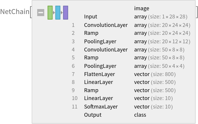
Retrieve the pre-trained net:

In[1]:=
NetModel["LeNet Trained on MNIST Data"]
Out[1]=

Basic usage

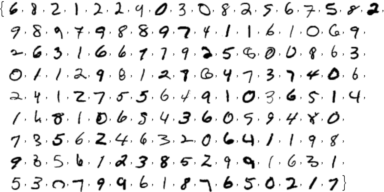
Apply the trained net to a set of inputs:

In[2]:=
NetModel["LeNet Trained on MNIST Data"][{\!\(\*
GraphicsBox[
TagBox[RasterBox[CompressedData["
1:eJxTTMoPSmNiYGAo5gASQYnljkVFiZXBAkBOaF5xZnpeaopnXklqemqRRRJI
mQwU/6cK2MHQhEtqiTTTJVxyQUy633BIneZSeolLWwSTBS6pP1ZM+bjkzjEJ
4ZL6X81kjkvqKydTHS65L0y45c4wMS3FJdfOxHRtcW3tkY/Y5cBA+T5WOaPk
5GgmJkNMOQWwW/6FMMliyqWB5X46MlliNTPo//+JTExbMOU+Ad0h683ElP8P
U+73fCGQM4XuYPHD//97LZmYLPdhlRrUAABgHMjK
"], {{0, 28}, {28, 0}}, {0, 255},
ColorFunction->GrayLevel],
BoxForm`ImageTag[
      "Byte", ColorSpace -> Automatic, Interleaving -> None],
Selectable->False],
DefaultBaseStyle->"ImageGraphics",
ImageSizeRaw->{28, 28},
PlotRange->{{0, 28}, {0, 28}}]\), \!\(\*
GraphicsBox[
TagBox[RasterBox[CompressedData["
1:eJxTTMoPSmNiYGAo5gASQYnljkVFiZXBAkBOaF5xZnpeaopnXklqemqRRRJI
mQwU/x9IsJWBKew2dql3okzMzH6/sMr5M7tPNGWeglXOQPf//yPiZdjlgMI7
mbHKVTOVQQkM8FCaef+v3dIih7HIfQphnnKCmdntBzYzdzKLizEzM+/DJvdD
hxnoP+xueafNxCvJwWSG3S0SV/+7M/tikbvAzHzyP1AOi5lvNJj9fwPlVJdj
ytUzMx8HUu7xWIw0ZdJ49f/PJUWTL5hyTMwT//+/xMxcgkUfE/Ou/92KzKGf
sMqpGLBzTb6MRer/Sh1gmGDzG/0AACEauS8=
"], {{0, 28}, {28, 0}}, {0, 255},
       
ColorFunction->GrayLevel],
BoxForm`ImageTag[
      "Byte", ColorSpace -> Automatic, Interleaving -> None],
Selectable->False],
DefaultBaseStyle->"ImageGraphics",
ImageSizeRaw->{28, 28},
PlotRange->{{0, 28}, {0, 28}}]\), \!\(\*
GraphicsBox[
TagBox[RasterBox[CompressedData["
1:eJxTTMoPSmNiYGAo5gASQYnljkVFiZXBAkBOaF5xZnpeaopnXklqemqRRRJI
mQwU/x9IsN/BdW1Vstx8LFK7eZgYmYBAcepvNJkvG/mZIHJMTLfR5OaBBAtX
r44CKqn4hSK1TRgoZQNipQEZp5ClPpoCRSr+gJiXgarykeWWAqUqoSalocrd
52ViCnwJMx5VLpeJyQVufyOK3Fo2JqYWOM+WiWkFkjZGRjs4p4mRkXE5nPcp
GegQGOeXM9BZ1vth3EAgT3I+lHMOyLE7Adf3y4uJqeY1hP3MFShXhbDuTwgT
0ywIa5s9Wnh+AnIFErYBgSVIRrz4G0LumxoTFIDiQaztPzLIQ5JzPogi9f+Z
NkzOof77fzTwY1EcSKps5y90GToCAMITbxU=
"], {{0, 28}, {28, 0}}, {0, 255},
       
ColorFunction->GrayLevel],
BoxForm`ImageTag[
      "Byte", ColorSpace -> Automatic, Interleaving -> None],
Selectable->False],
DefaultBaseStyle->"ImageGraphics",
ImageSizeRaw->{28, 28},
PlotRange->{{0, 28}, {0, 28}}]\)}]
Out[2]=

Give class probabilities for a single input:
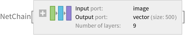
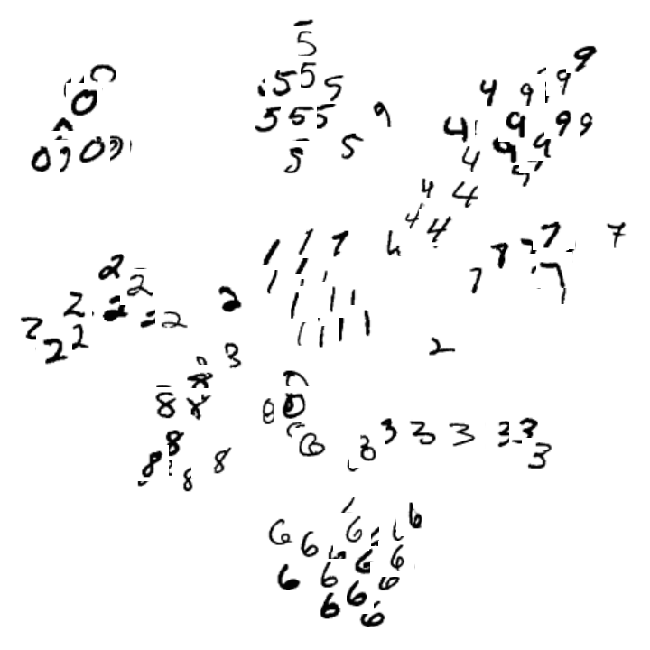
In[3]:=
NetModel["LeNet Trained on MNIST Data"][\!\(\*
GraphicsBox[
TagBox[RasterBox[CompressedData["
1:eJxTTMoPSmNiYGAo5gASQYnljkVFiZXBAkBOaF5xZnpeaopnXklqemqRRRJI
mQwU/x9IsJWBKew2dql3okzMzH6/sMr5M7tPNGWeglXOQPf//yPiZdjlgMI7
mbHKVTOVQQkM8FCaef+v3dIih7HIfQphnnKCmdntBzYzdzKLizEzM+/DJvdD
hxnoP+xueafNxCvJwWSG3S0SV/+7M/tikbvAzHzyP1AOi5lvNJj9fwPlVJdj
ytUzMx8HUu7xWIw0ZdJ49f/PJUWTL5hyTMwT//+/xMxcgkUfE/Ou/92KzKGf
sMqpGLBzTb6MRer/Sh1gmGDzG/0AACEauS8=
"], {{0, 28}, {28, 0}}, {0, 255},
      
ColorFunction->GrayLevel],
BoxForm`ImageTag[
     "Byte", ColorSpace -> Automatic, Interleaving -> None],
Selectable->False],
DefaultBaseStyle->"ImageGraphics",
ImageSizeRaw->{28, 28},
PlotRange->{{0, 28}, {0, 28}}]\), "Probabilities"]
Out[3]=

Feature extraction

Create a subset of the MNIST dataset:

In[4]:=
sample = Keys[RandomSample[ResourceData["MNIST"], 150]]
Out[4]=

Remove the last linear layer of the net, which will be used as a feature extractor:

In[5]:=
extractor = Take[NetModel["LeNet Trained on MNIST Data"], {1, -3}]
Out[5]=

Visualize the features of a subset of the MNIST dataset:

In[6]:=
FeatureSpacePlot[sample, FeatureExtractor -> extractor]
Out[6]=

Visualization of net operation

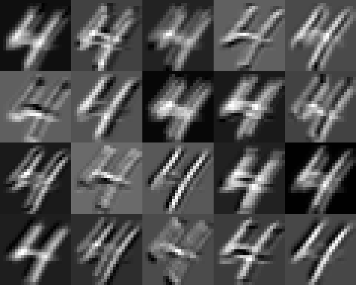
Extract the convolutional features from the first layer:

In[7]:=
convFeatures = NetModel["LeNet Trained on MNIST Data"][\!\(\*
GraphicsBox[
TagBox[RasterBox[CompressedData["
1:eJxTTMoPSmNiYGAo5gASQYnljkVFiZXBAkBOaF5xZnpeaopnXklqemqRRRJI
mQwU/x+sYDHDDlxSN7jtoKw9McdRpf6EMC6HsLZxFn9GlVvEGP4PzHjM6/AX
Veo6p+oXMOOnifA7NCk5ZoiJv+MYJ6FK/YtgnANhlTC6/kSR+lbKGPkb4lhW
6Zeo2rIYGbNqWq8AWa6sB1Gl+lgYGRkNGNniZqWz5KNKXRBkYCoD+mi9Lzsj
46bnv5Hl1nCHzwYzPjgwhtfWXkHRCFM6hzEcRRMSuKXEdxuH1P+ljKm4pN4p
ilzAJbeGMQOX1E8Ribu45JYzeuCS+l/KfQCnHNUAAFQtzfI=
"], {{0, 28}, {28, 0}}, {0, 255},
ColorFunction->GrayLevel],
BoxForm`ImageTag[
      "Byte", ColorSpace -> Automatic, Interleaving -> None],
Selectable->False],
DefaultBaseStyle->"ImageGraphics",
ImageSizeRaw->{28, 28},
PlotRange->{{0, 28}, {0, 28}}]\), NetPort[1, "Output"]]
Out[7]=

Visualize the features:

In[8]:=
ImageCollage[Map[ImageAdjust@*Image, convFeatures], ImageSize -> Medium]
Out[8]=

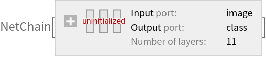
Training the uninitialized architecture

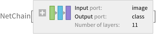
Retrieve the uninitialized architecture:

In[9]:=
net = NetModel["LeNet Trained on MNIST Data", "UninitializedEvaluationNet"]
Out[9]=

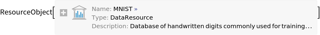
Retrieve the MNIST dataset:

In[10]:=
mnist = ResourceObject["MNIST"]
Out[10]=

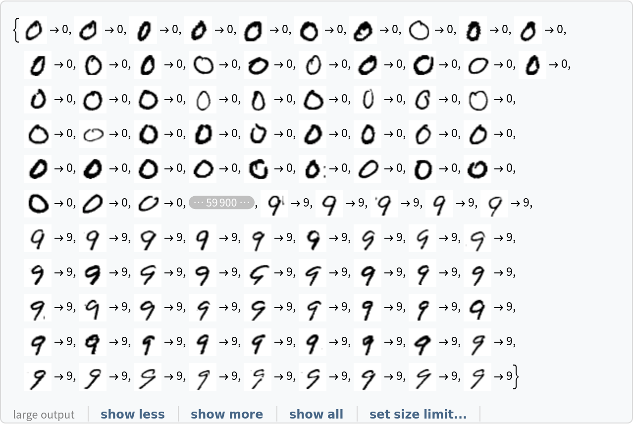
Use the training dataset provided:

In[11]:=
trainSet = ResourceData[mnist, "TrainingData"]
Out[11]=

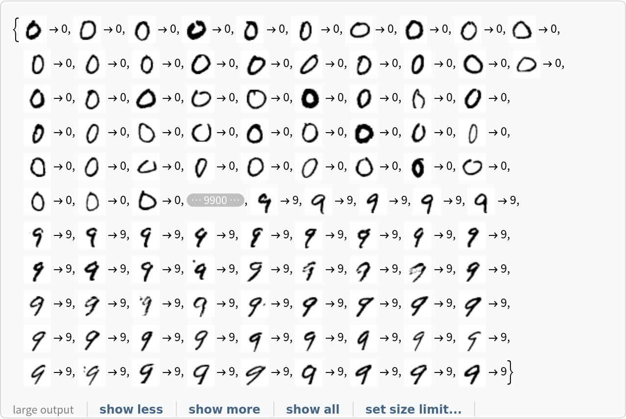
Use the test dataset provided:

In[12]:=
valSet = ResourceData[mnist, "TestData"]
Out[12]=

Train the net:

In[13]:=
trained = NetTrain[net, trainSet, ValidationSet -> valSet]
Out[13]=

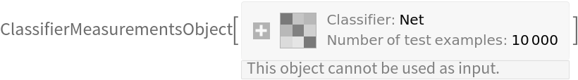
Generate a ClassifierMeasurementsObject of the net with the test set:

In[14]:=
cm = ClassifierMeasurements[trained, valSet]
Out[14]=

Evaluate the accuracy on the validation set:

In[15]:=
cm["Accuracy"]
Out[15]=

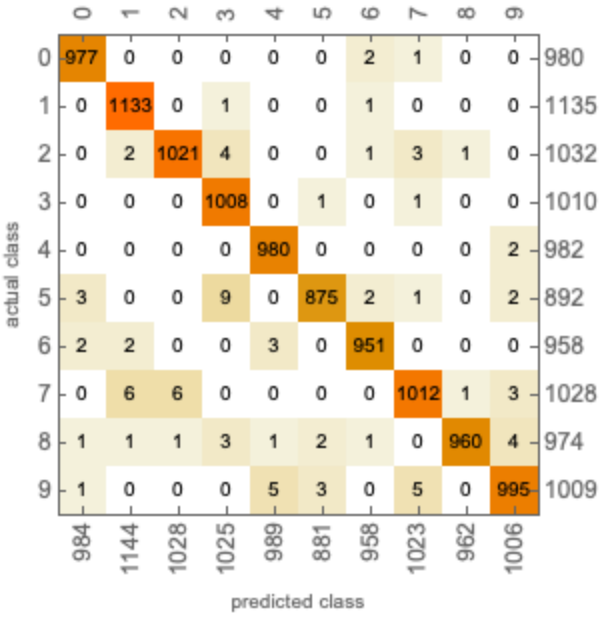
Visualize the confusion matrix:

In[16]:=
cm["ConfusionMatrixPlot"]
Out[16]=

Net information

Inspect the number of parameters of all arrays in the net:

In[17]:=
NetInformation[
 NetModel["LeNet Trained on MNIST Data"], "ArraysElementCounts"]
Out[17]=

Obtain the total number of parameters:

In[18]:=
NetInformation[
 NetModel["LeNet Trained on MNIST Data"], "ArraysTotalElementCount"]
Out[18]=

Obtain the layer type counts:

In[19]:=
NetInformation[
 NetModel["LeNet Trained on MNIST Data"], "LayerTypeCounts"]
Out[19]=

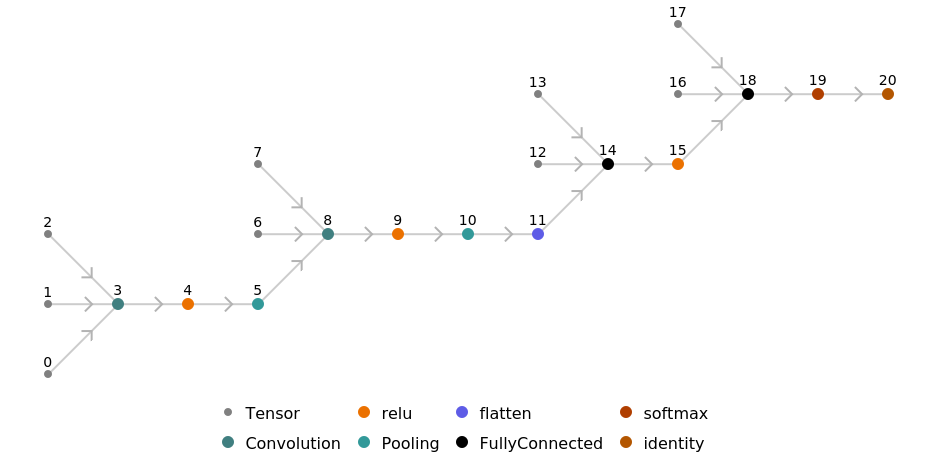
Display the summary graphic:

In[20]:=
NetInformation[
 NetModel["LeNet Trained on MNIST Data"], "SummaryGraphic"]
Out[20]=

Export to MXNet

Export the net into a format that can be opened in MXNet:

In[21]:=
jsonPath = Export[FileNameJoin[{$TemporaryDirectory, "net.json"}], NetModel["LeNet Trained on MNIST Data"], "MXNet"]
Out[21]=

Export also creates a net.params file containing parameters:

In[22]:=
paramPath = FileNameJoin[{DirectoryName[jsonPath], "net.params"}]
Out[22]=

Get the size of the parameter file:

In[23]:=
FileByteCount[paramPath]
Out[23]=

The size is similar to the byte count of the resource object:

In[24]:=
ResourceObject["LeNet Trained on MNIST Data"]["ByteCount"]
Out[24]=

Represent the MXNet net as a graph:

In[25]:=
Import[jsonPath, {"MXNet", "NodeGraphPlot"}]
Out[25]=

Requirements

Wolfram Language 11.1 (March 2017) or above

Resource History

Reference

  • Y. LeCun, L. Bottou, Y. Bengio, P. Haffner, "Gradient-Based Learning Applied to Document Recognition," Proceedings of the IEEE, 86(11), 2278-2324 (1998)
  • Available from: http://yann.lecun.com/exdb/lenet